library(ggplot2)
library(patchwork)

te_paper  <- "#f5f4ee"
te_ink    <- "#16241d"
te_body   <- "#2c3a31"
te_forest <- "#275139"
te_rust   <- "#b5534e"
te_gold   <- "#c9b458"
te_line   <- "#dad9ca"

theme_datasheet <- function() {
  theme_minimal(base_size = 12) +
    theme(plot.background  = element_rect(fill = te_paper, colour = NA),
          panel.background = element_rect(fill = te_paper, colour = NA),
          panel.grid.major = element_line(colour = te_line, linewidth = 0.3),
          panel.grid.minor = element_blank(),
          text             = element_text(colour = te_body),
          plot.title       = element_text(colour = te_ink, face = "bold"),
          plot.subtitle    = element_text(colour = te_body),
          axis.text        = element_text(colour = te_body))
}
rule_cols <- c(Poisson = te_rust, `quasi-Poisson` = te_gold,
`negative binomial` = te_forest, `true model` = te_ink)Detecting a die-off from carcass reports
R
surveillance
wildlife disease
negative binomial
simulation
ecology tutorial
A historical-limits alarm on weekly carcass reports: the variance model sets the real false alarm rate, and decides detection when noise varies by season. In R.
A regional wildlife health scheme asks walkers, wardens and farmers to report dead birds and mammals through a web form. The reports are tallied by week. Most weeks bring a handful: a road-killed badger, a gull on the tideline, a pigeon under a window. A die-off from avian influenza, botulism or a pesticide spill arrives in the same stream as a burst of extra carcasses, and the scheme wants a rule that flags the burst in the week it happens without somebody reading every report. A rule many public health surveillance systems use for this is the historical-limits alarm: compare this week’s count with the same weeks in previous years and raise an alarm when the count sits above an upper limit computed from them.
Farrington and colleagues built that alarm for the weekly laboratory reports of infectious disease in England and Wales, and it has been refined and reviewed since (Unkel and colleagues give the survey; Noufaily and colleagues the improved version). Its limit needs a model for how much a weekly count varies when nothing is happening. A Poisson limit assumes the variance equals the mean. Carcass reports do not behave like that: a sunny bank holiday puts more walkers on the footpaths, a local news story brings a flurry of reports, a wet week brings almost none, and all of that multiplies the count before a single extra animal has died. That a Poisson limit raises too many alarms when the counts are overdispersed is textbook, and it is the reason the original algorithm used a quasi-Poisson dispersion. This post demonstrates it only briefly. The part it measures is what happens next: the dispersion has to be estimated from a few dozen historical weeks, a limit whose false alarm rate is right misses a large share of moderate die-offs, and whether the variance model also changes how well the alarm separates a die-off from a noisy week depends on how much the dispersion of the counts changes through the year.
The neighbours on this site price related alarms. Testing a monitoring series every year measures how repeated looks at a slow population trend inflate the false alarm rate of a test that is correct at a single look. Reference sites and tolerance bounds sets a threshold on a continuous index from a small reference sample and shows that the false alarm rate belongs to the reference set that was drawn. Dispersion checks when the counts are small measures how well the usual overdispersion statistics behave at low counts. And carcass searches and fatality estimates is about how many carcasses a searcher finds, not about alarms. Here the threshold is on a weekly count, and the post separates two jobs of the variance model: setting the false alarm rate, and following a dispersion that changes from season to season.
The post sets up the alarm and three limits, measures the false alarm rate as reporting noise grows, looks at how well thirty five historical weeks pin down a dispersion, measures detection and shows that under one level of noise all year the three limits trade false alarms for detection along nearly the same curve, then lets the noise and the mean change with the season to see when the curves separate, and finally puts past die-offs into the baseline to see what down-weighting them does.
One alarm, three limits
The reporting system in the simulation has a seasonal mean of six carcasses a week, rising to nine in early spring and falling to three in autumn. Each week’s reporting effort multiplies that mean by a lognormal factor with mean one and log-scale standard deviation s, and the count is Poisson given the product. With s equal to zero the reports are pure Poisson. With s equal to 0.6, a week at half or one and a half times the usual reporting effort is within one standard deviation of normal, which is not an extreme assumption for a scheme that depends on the public.
The alarm for week t of the current year uses the counts from weeks t - 3 to t + 3 in each of the five previous years: thirty five historical weeks. The Farrington algorithm builds its baseline the same way, from a chosen number of previous years and a chosen number of weeks either side of the current one. The baseline mean is the average of the thirty five counts and the dispersion is the Pearson statistic divided by its degrees of freedom (what an intercept-only quasi-Poisson fit reports), floored at one as in Farrington’s algorithm. Three limits are then computed from the same two numbers.
The Poisson limit is the upper quantile of a Poisson distribution with the baseline mean. The quasi-Poisson limit is Farrington’s: a normal limit on the two-thirds power of the count, which corrects the skewness of small counts, with the variance of the prediction included through a factor of one plus one over thirty five. The negative binomial limit is the upper quantile of a negative binomial with the baseline mean and a size chosen so its variance is the dispersion times the mean; a plug-in negative binomial quantile of this kind is one of the threshold options in the surveillance package’s implementation of the improved algorithm of Noufaily and colleagues. Each limit is set at a one-sided level of 0.005 per week, and weeks 4 to 49 are tested, so the nominal false alarm rate is 46 times 0.005 per year. A fourth limit, the true model, uses the true seasonal mean and a negative binomial with the true variance. No real scheme has it; it marks what the noise alone allows.
alpha_wk <- 0.005                     # one-sided level per tested week
n_back   <- 5                         # historical years
half_win <- 3                         # weeks either side of the tested week
wk_all   <- 1:52
test_wk  <- (1 + half_win):(52 - half_win)
n_test   <- length(test_wk)
fa_nominal <- n_test * alpha_wk
die_len  <- 2                         # die-off lasts two weeks

base_mu <- function(w, seasonal = TRUE) {
  if (seasonal) 6 * (1 + 0.5 * sin(2 * pi * w / 52)) else rep(6, length(w))
}

# counts: array rep x year x week; past die-offs only in historical years
# s_week and mu_week (length 52) override the constant noise and the mean
sim_reports <- function(n_rep, n_yr, s_rep, seasonal = TRUE,
                        past_D = 0, past_prob = 0,
                        s_week = NULL, mu_week = NULL) {
  s_vec  <- if (is.null(s_week)) rep(s_rep, 52) else s_week
  mu_vec <- if (is.null(mu_week)) base_mu(wk_all, seasonal) else mu_week
  counts <- eff <- array(0, c(n_rep, n_yr, 52))
  for (yr in 1:n_yr) {
    mu_mat <- matrix(mu_vec, n_rep, 52, byrow = TRUE)
    if (past_D > 0 && yr < n_yr) {
      hit <- which(runif(n_rep) < past_prob)
      onset <- sample(1:51, length(hit), replace = TRUE)
      for (k in 0:1) {
        ix <- cbind(hit, onset + k)
        mu_mat[ix] <- mu_mat[ix] + past_D / die_len
      }
    }
    e_mat <- matrix(exp(rnorm(n_rep * 52, rep(-s_vec^2 / 2, each = n_rep),
                              rep(s_vec, each = n_rep))), n_rep, 52)
    counts[, yr, ] <- matrix(rpois(n_rep * 52, mu_mat * e_mat), n_rep, 52)
    eff[, yr, ] <- e_mat
  }
  list(counts = counts, eff = eff)
}

# baseline mean and dispersion for every rep x tested week,
# with optional Farrington reweighting at a residual cut-off
baseline_fit <- function(hist_counts, cutoff = Inf) {
  n_rep <- dim(hist_counts)[1]
  n_b   <- dim(hist_counts)[2] * (2 * half_win + 1)
  m_out <- phi_out <- matrix(NA_real_, n_rep, n_test)
  for (j in seq_len(n_test)) {
    w <- test_wk[j]
    h <- matrix(hist_counts[, , (w - half_win):(w + half_win)], n_rep, n_b)
    m <- rowMeans(h)
    phi <- pmax(1, rowSums((h - m)^2 / m) / (n_b - 1))
    if (is.finite(cutoff)) {
      s_ans <- 1.5 * (h^(2 / 3) - m^(2 / 3)) /
        (m^(1 / 6) * sqrt(phi * (1 - 1 / n_b)))
      wt <- ifelse(s_ans > cutoff, s_ans^-2, 1)
      wt <- wt * n_b / rowSums(wt)
      m <- rowSums(wt * h) / n_b
      phi <- pmax(1, rowSums(wt * (h - m)^2 / m) / (n_b - 1))
    }
    m_out[, j] <- m
    phi_out[, j] <- phi
  }
  list(m = m_out, phi = phi_out, n_b = n_b)
}

# upper-tail p values: an alarm at level a is p <= a for every rule
alarm_p <- function(cur, fit, true_m, s_mat) {
  m <- fit$m
  phi <- fit$phi
  z_q <- 1.5 * ((cur / m)^(2 / 3) - 1) / sqrt(phi * (1 + 1 / fit$n_b) / m)
  size_nb <- ifelse(phi > 1, m / (phi - 1), 1e8)
  size_true <- ifelse(s_mat > 0, true_m / (true_m * (exp(s_mat^2) - 1)), 1e8)
  list(`Poisson` = ppois(cur - 1, m, lower.tail = FALSE),
       `quasi-Poisson` = pnorm(z_q, lower.tail = FALSE),
       `negative binomial` = pnbinom(cur - 1, size = size_nb, mu = m,
                                     lower.tail = FALSE),
       `true model` = pnbinom(cur - 1, size = size_true, mu = true_m,
                              lower.tail = FALSE))
}

run_cell <- function(n_rep, s_rep, seasonal = TRUE, n_hist = n_back,
                     cutoff = Inf, past_D = 0, past_prob = 0,
                     D_set = c(10, 25, 50), s_week = NULL, mu_week = NULL) {
  sim <- sim_reports(n_rep, n_hist + 1, s_rep, seasonal, past_D, past_prob,
                     s_week, mu_week)
  fit <- baseline_fit(sim$counts[, 1:n_hist, , drop = FALSE], cutoff)
  cur <- sim$counts[, n_hist + 1, test_wk]
  eff <- sim$eff[, n_hist + 1, test_wk]
  mu_vec <- if (is.null(mu_week)) base_mu(wk_all, seasonal) else mu_week
  s_vec  <- if (is.null(s_week)) rep(s_rep, 52) else s_week
  true_m <- matrix(mu_vec[test_wk], n_rep, n_test, byrow = TRUE)
  s_mat  <- matrix(s_vec[test_wk], n_rep, n_test, byrow = TRUE)
  p_null <- alarm_p(cur, fit, true_m, s_mat)
  onset <- sample(1:(n_test - 1), n_rep, replace = TRUE)
  ix1 <- cbind(1:n_rep, onset)
  ix2 <- cbind(1:n_rep, onset + 1)
  p_die <- lapply(D_set, function(D) {
    cur_d <- cur
    for (ix in list(ix1, ix2)) {
      cur_d[ix] <- cur_d[ix] + rpois(n_rep, D / die_len * eff[ix])
    }
    pd <- alarm_p(cur_d, fit, true_m, s_mat)
    lapply(pd, function(p) cbind(first = p[ix1], either = pmin(p[ix1], p[ix2])))
  })
  names(p_die) <- D_set
  list(p_null = p_null, p_die = p_die, phi = fit$phi, m = fit$m, cur = cur, onset = onset)
}

fa_rate  <- function(p, a = alpha_wk) mean(rowSums(p <= a))
any_rate <- function(p, a = alpha_wk) mean(rowSums(p <= a) > 0)
det_rate <- function(pd, a = alpha_wk) mean(pd[, "either"] <= a)
rule_names <- c("Poisson", "quasi-Poisson", "negative binomial", "true model")
The nominal rate is 0.23 false alarms a year. A die-off adds D carcasses spread evenly over two consecutive tested weeks, and its extra reports are subject to the same weekly reporting effort as the background. It counts as detected when either of its two weeks raises an alarm. All of these constants were fixed before the first run.
set.seed(3107)
demo <- sim_reports(1, n_back + 1, 0.6)
demo_fit <- baseline_fit(demo$counts[, 1:n_back, , drop = FALSE])
demo_cur <- demo$counts[1, n_back + 1, ]
demo_cur[30:31] <- demo_cur[30:31] +
  rpois(2, 25 / die_len * demo$eff[1, n_back + 1, 30:31])
m_d <- demo_fit$m[1, ]
phi_d <- demo_fit$phi[1, ]
z_a <- qnorm(1 - alpha_wk)
lim_df <- rbind(
  data.frame(week = test_wk, limit = qpois(1 - alpha_wk, m_d), rule = "Poisson"),
  data.frame(week = test_wk, rule = "quasi-Poisson",
             limit = m_d * (1 + (2 / 3) * z_a *
                              sqrt(phi_d * (1 + 1 / demo_fit$n_b) / m_d))^1.5),
  data.frame(week = test_wk, rule = "negative binomial",
             limit = qnbinom(1 - alpha_wk, mu = m_d,
                             size = ifelse(phi_d > 1, m_d / (phi_d - 1), 1e8))))
lim_df$rule <- factor(lim_df$rule, levels = rule_names[1:3])
cur_df <- data.frame(week = wk_all, count = demo_cur,
                     die = wk_all %in% 30:31)
demo_bg <- !(test_wk %in% 30:31)
demo_fa <- tapply(demo_cur[test_wk][demo_bg] > lim_df$limit[rep(demo_bg, 3)],
                  lim_df$rule[rep(demo_bg, 3)], sum)
demo_hit <- tapply(demo_cur[test_wk][!demo_bg] > lim_df$limit[rep(!demo_bg, 3)],
                   lim_df$rule[rep(!demo_bg, 3)], sum)
demo_max <- max(demo_cur[test_wk][demo_bg])

ggplot(cur_df, aes(week, count)) +
  geom_col(aes(fill = die), width = 0.8) +
  geom_step(data = lim_df, aes(week, limit, colour = rule),
            linewidth = 0.9, direction = "mid") +
  scale_fill_manual(values = c(`FALSE` = te_line, `TRUE` = te_body),
                    labels = c("background week", "die-off week"), name = NULL) +
  scale_colour_manual(values = rule_cols, name = NULL) +
  labs(x = "week of the current year", y = "carcass reports",
       title = "Three limits from the same thirty five weeks",
       subtitle = "an alarm is a column above a line") +
  theme_datasheet() +
  theme(legend.position = "bottom", legend.box = "vertical")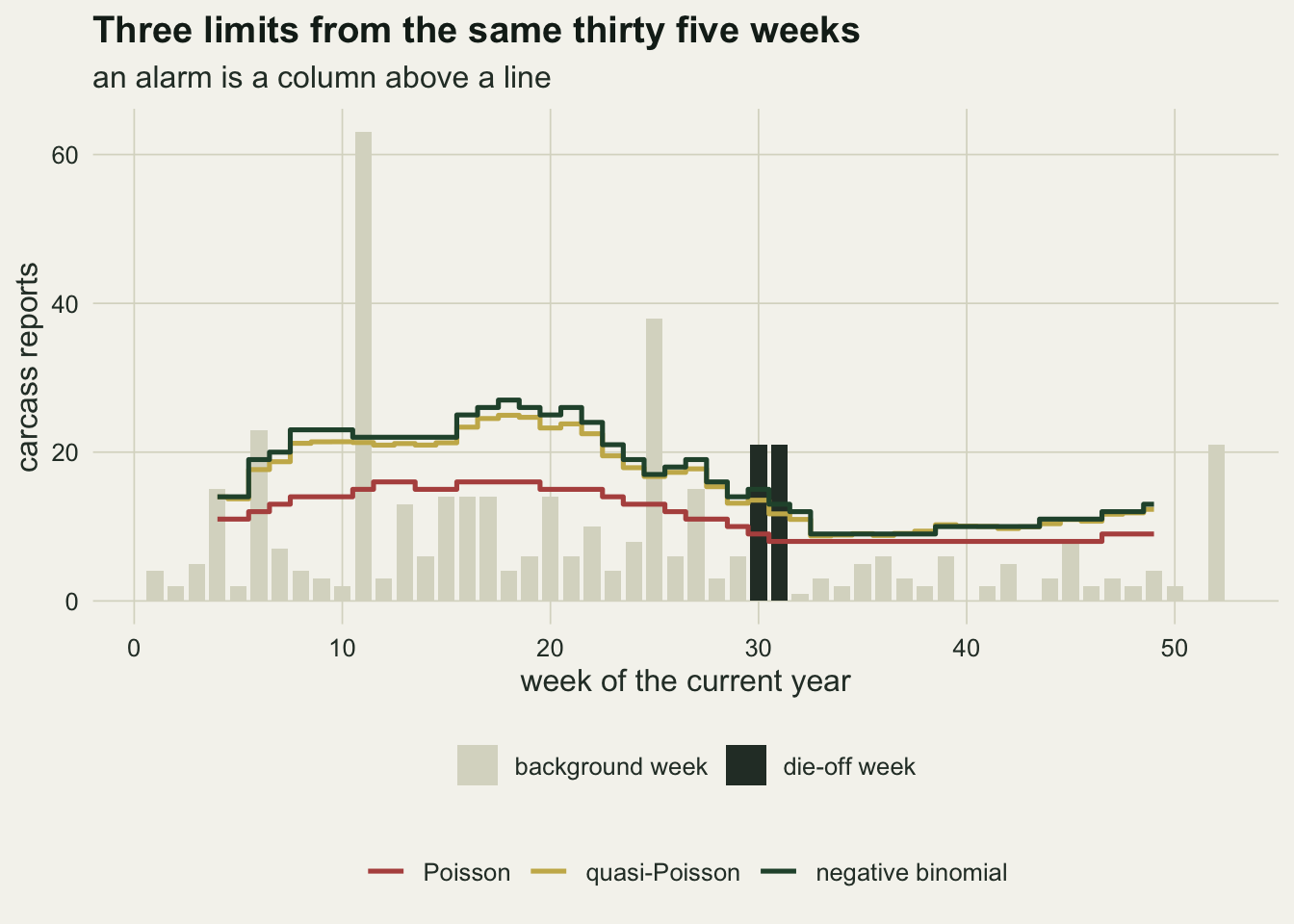
The figure is one year and proves nothing on its own; it shows what the rules look like. This year happens to be a rough one: its largest background week brought 63 reports, and among the background weeks the Poisson, quasi-Poisson and negative binomial limits are crossed 5, 4 and 4 times, while the two die-off weeks cross them 2, 2 and 2 times. The limits move with the season because the baseline does, and they jump from week to week because each week’s baseline is a different set of thirty five noisy counts. The next section measures what happens over thousands of years.
The rate is right only with the right variance
n_rep  <- 4000
s_grid <- c(0, 0.15, 0.3, 0.45, 0.6)
s_use  <- 0.6
set.seed(5501)
cells <- lapply(s_grid, function(s) run_cell(n_rep, s))
names(cells) <- s_grid

fa_tab <- do.call(rbind, lapply(seq_along(s_grid), function(i) {
  data.frame(s = s_grid[i], rule = rule_names,
             fa = sapply(cells[[i]]$p_null, fa_rate),
             fa_se = sapply(cells[[i]]$p_null, function(p)
               sd(rowSums(p <= alpha_wk)) / sqrt(n_rep)),
             any_fa = sapply(cells[[i]]$p_null, any_rate))
}))
fa_at <- function(s, r, col = "fa") fa_tab[fa_tab$s == s & fa_tab$rule == r, col]
fa_se_max <- max(fa_tab$fa_se)
pois_mult <- fa_at(s_use, "Poisson") / fa_nominal
nb_mult   <- fa_at(s_use, "negative binomial") / fa_nominal

set.seed(5502)
flat_cell <- run_cell(n_rep, s_use, seasonal = FALSE)
fa_flat <- sapply(flat_cell$p_null, fa_rate)
Each cell is 4000 simulated years with their own five-year history, so the Monte Carlo standard error of a false alarm rate is at most 0.027 alarms a year.
With pure Poisson reports the Poisson limit gives 0.17 false alarms a year, the quasi-Poisson limit 0.16 and the negative binomial limit 0.12, against the nominal 0.23. All three sit below it, because a discrete count cannot hit the level exactly and the next count up is always on the safe side, and the estimated dispersion, floored at one, can only widen the quasi-Poisson and negative binomial limits.
At s = 0.6 the Poisson limit raises 3.01 false alarms a year, 13.1 times the nominal rate, and 96 per cent of years carry at least one. That is the textbook result and the reason Farrington’s algorithm estimated a dispersion. The quasi-Poisson limit brings the rate down to 0.77 and the negative binomial limit to 0.53, which is still 2.3 times nominal. Even the true model gives 0.29, because the reporting noise is lognormal and a negative binomial with the right mean and variance still has a slightly thinner far tail.
The seasonal mean is not what drives these numbers. With a flat mean of six a week and the same noise, the four rules give 3.04, 0.77, 0.55 and 0.27 false alarms a year. A seven-week window on this season adds little variance to the baseline compared with the reporting noise.
fa_tab$rule <- factor(fa_tab$rule, levels = rule_names)
ggplot(fa_tab, aes(s, fa, colour = rule)) +
  geom_hline(yintercept = fa_nominal, linetype = "dashed",
             colour = te_body, linewidth = 0.6) +
  geom_line(linewidth = 0.9) +
  geom_point(size = 2.2) +
  scale_colour_manual(values = rule_cols, name = NULL) +
  scale_y_log10() +
  labs(x = "reporting noise s (log-scale standard deviation)",
       y = "false alarms per year (log scale)",
       title = "Only a variance model buys back the rate",
       subtitle = paste0("dashed: nominal ", sprintf("%.2f", fa_nominal),
                         " per year; 46 tested weeks at level 0.005")) +
  theme_datasheet() +
  theme(legend.position = "bottom")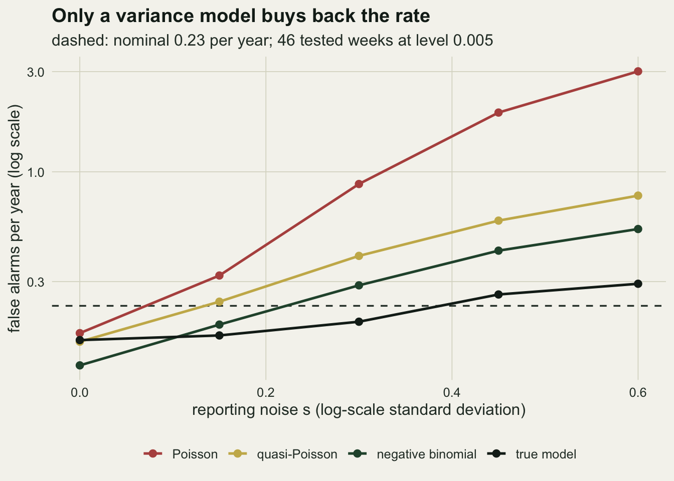
Thirty five weeks is a short record for a dispersion
The negative binomial limit is right in form and still over-alarms, and the gap to the true model is estimation. A dispersion is a variance ratio, and thirty five counts do not pin a variance down.
phi_true_flat <- 1 + 6 * (exp(s_use^2) - 1)
phi_hat <- as.vector(flat_cell$phi)
phi_q <- quantile(phi_hat, c(0.05, 0.5, 0.95))
share_low <- mean(phi_hat < phi_true_flat)

nb_alarm <- flat_cell$p_null[["negative binomial"]] <= alpha_wk
phi_low  <- flat_cell$phi < phi_true_flat
share_fa_low <- sum(nb_alarm & phi_low) / sum(nb_alarm)
rate_low  <- mean(nb_alarm[phi_low])
rate_high <- mean(nb_alarm[!phi_low])

# swap in the true mean or the true dispersion, one at a time
fa_nb_swap <- function(mu, phi) {
  size_sw <- ifelse(phi > 1, mu / (phi - 1), 1e8)
  mean(rowSums(pnbinom(flat_cell$cur - 1, size = size_sw, mu = mu,
                       lower.tail = FALSE) <= alpha_wk))
}
fa_estm_truephi <- fa_nb_swap(flat_cell$m, phi_true_flat)
fa_truem_estphi <- fa_nb_swap(6, flat_cell$phi)

set.seed(5503)
long_cell <- run_cell(n_rep, s_use, n_hist = 10)
fa_long <- sapply(long_cell$p_null, fa_rate)
On the flat control the true dispersion is 3.60. The estimate from thirty five weeks has a median of 3.22 and a central ninety per cent range from 1.86 to 6.16; 63 per cent of baselines put it below the truth. The Pearson estimate of a lognormal-Poisson variance is skewed: a few large counts push it up, and their absence leaves it low.
The alarms come from the low side. Weeks whose baseline underestimated the dispersion raise a false alarm with probability 0.0171, weeks whose baseline overestimated it with probability 0.0032, and the low weeks carry 90 per cent of all the negative binomial false alarms (against 63 per cent of the baselines). A low dispersion estimate tends to come with a low mean estimate, so the two are separated by swapping in the truth one at a time: on the same simulated years the negative binomial limit gives 0.55 false alarms a year, 0.30 with the estimated mean and the true dispersion, and 0.48 with the true mean and the estimated dispersion. The dispersion is the larger part. The mechanism is not symmetric, so the errors do not cancel: a limit that is too low by some margin adds more alarms than the same margin too high removes.
Doubling the history shrinks the excess but does not remove it. With ten previous years, seventy weeks in each baseline, the negative binomial limit raises 0.40 false alarms a year against 0.53 with five and 0.29 for the true model, and the Poisson limit, which has nothing to estimate beyond the mean, stays at 2.96.
phi_df <- data.frame(phi = phi_hat[phi_hat < quantile(phi_hat, 0.995)])
ggplot(phi_df, aes(phi)) +
  geom_histogram(binwidth = 0.25, boundary = 1, fill = te_forest, colour = te_paper) +
  geom_vline(xintercept = phi_true_flat, colour = te_rust,
             linetype = "dashed", linewidth = 0.8) +
  labs(x = "estimated dispersion (Pearson statistic over df, floored at one)",
       y = "baselines",
       title = "The dispersion is the noisy input",
       subtitle = "dashed red: the true dispersion; top half per cent of estimates not drawn") +
  theme_datasheet()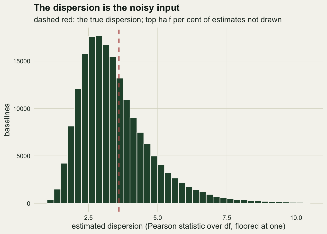
The price is detection, at one level of noise
det_tab <- do.call(rbind, lapply(c("0", "0.6"), function(s) {
  do.call(rbind, lapply(names(cells[[s]]$p_die), function(D) {
    data.frame(s = as.numeric(s), D = as.numeric(D), rule = rule_names,
               det = sapply(cells[[s]]$p_die[[D]], det_rate))
  }))
}))
det_at <- function(s, D, r) det_tab$det[det_tab$s == s & det_tab$D == D & det_tab$rule == r]
det_se_max <- sqrt(0.25 / n_rep)

first_share <- sapply(cells[["0.6"]]$p_die[["25"]], function(pd)
  mean(pd[, "first"] <= alpha_wk) / mean(pd[, "either"] <= alpha_wk))

a_grid <- 10^seq(-30, -0.7, by = 0.1)
roc_df <- do.call(rbind, lapply(rule_names, function(r) {
  data.frame(rule = r, a = a_grid,
             fa = sapply(a_grid, function(a) fa_rate(cells[["0.6"]]$p_null[[r]], a)),
             det = sapply(a_grid, function(a) det_rate(cells[["0.6"]]$p_die[["25"]][[r]], a)))
}))
det_matched <- function(r, target, roc = roc_df) {
  roc_sub <- roc[roc$rule == r & roc$fa > 0, ]
  approx(log(roc_sub$fa), roc_sub$det, xout = log(target), ties = mean)$y
}
fa_pois_use <- fa_at(s_use, "Poisson")
match_nom  <- sapply(rule_names, det_matched, target = fa_nominal)
match_pois <- sapply(rule_names, det_matched, target = fa_pois_use)
At s = 0 every limit finds almost every die-off of 25 carcasses: 0.98 for Poisson and 0.97 for the negative binomial. At s = 0.6 the same die-off is detected with probability 0.83 by the Poisson limit, 0.57 by the quasi-Poisson limit, 0.50 by the negative binomial limit and 0.48 by the true model. A die-off of 10 carcasses is found 0.19 of the time by the negative binomial limit, and one of 50 0.80. Monte Carlo standard errors of these proportions are at most 0.008.
So the limit that comes closest to its stated false alarm rate misses 50 per cent of 25-carcass die-offs that the Poisson limit mostly catches. Read that way the Poisson limit looks like the better tool. The right panel below says otherwise. Sweeping the level of each rule traces how many false alarms it must accept for a given detection. At the Poisson limit’s own rate of 3.01 false alarms a year, the quasi-Poisson and negative binomial rules detect 0.80 and 0.81 against the Poisson’s 0.83. At the nominal 0.23 a year, they detect 0.39 and 0.37, the Poisson rule 0.38 and the true model 0.44. Estimating the baseline from thirty five noisy weeks costs a few points of detection against the true model at the same rate; which distribution is used costs almost nothing once the rate is matched.
With one level of reporting noise all year, the rules do not differ much in how well they separate a die-off from a noisy week. They differ in where they sit on the curve, and the Poisson limit sits far up it without saying so. What the variance model buys is an honest statement of the operating point, and at an honest rate of a fraction of an alarm a year this reporting noise lets a scheme find a 25-carcass die-off in fewer than half of the years it happens.
Of the 25-carcass die-offs the negative binomial limit does detect at level 0.005, 63 per cent are flagged in their first week; for the Poisson limit the share is 72 per cent.
det_tab$rule <- factor(det_tab$rule, levels = rule_names)
det_tab$noise <- factor(ifelse(det_tab$s == 0, "pure Poisson reports", "reporting noise s = 0.6"),
                        levels = c("pure Poisson reports", "reporting noise s = 0.6"))
p_det <- ggplot(det_tab, aes(D, det, colour = rule)) +
  geom_line(linewidth = 0.8) +
  geom_point(size = 2) +
  facet_wrap(~ noise, ncol = 1) +
  scale_colour_manual(values = rule_cols, name = NULL) +
  scale_x_continuous(breaks = c(10, 25, 50)) +
  scale_y_continuous(limits = c(0, 1)) +
  labs(x = "extra carcasses over two weeks", y = "probability of detection",
       title = "Detection at level 0.005") +
  theme_datasheet() +
  theme(legend.position = "none")

roc_df$rule <- factor(roc_df$rule, levels = rule_names)
pt_df <- data.frame(rule = factor(rule_names, levels = rule_names),
                    fa = fa_tab$fa[fa_tab$s == s_use],
                    det = det_tab$det[det_tab$s == s_use & det_tab$D == 25])
p_roc <- ggplot(roc_df[roc_df$fa > 0.01 & roc_df$fa < 12, ], aes(fa, det, colour = rule)) +
  geom_vline(xintercept = fa_nominal, linetype = "dashed",
             colour = te_body, linewidth = 0.6) +
  geom_line(linewidth = 0.9) +
  geom_point(data = pt_df, size = 3) +
  scale_colour_manual(values = rule_cols, name = NULL) +
  scale_x_log10() +
  scale_y_continuous(limits = c(0, 1)) +
  labs(x = "false alarms per year (log scale)", y = "detection of 25 carcasses",
       title = "One noise level: one curve, different points",
       subtitle = "points: level 0.005; dashed: nominal rate") +
  theme_datasheet() +
  theme(legend.position = "bottom")

p_det + p_roc + plot_layout(widths = c(1, 1.4)) +
  plot_annotation(theme = theme_datasheet())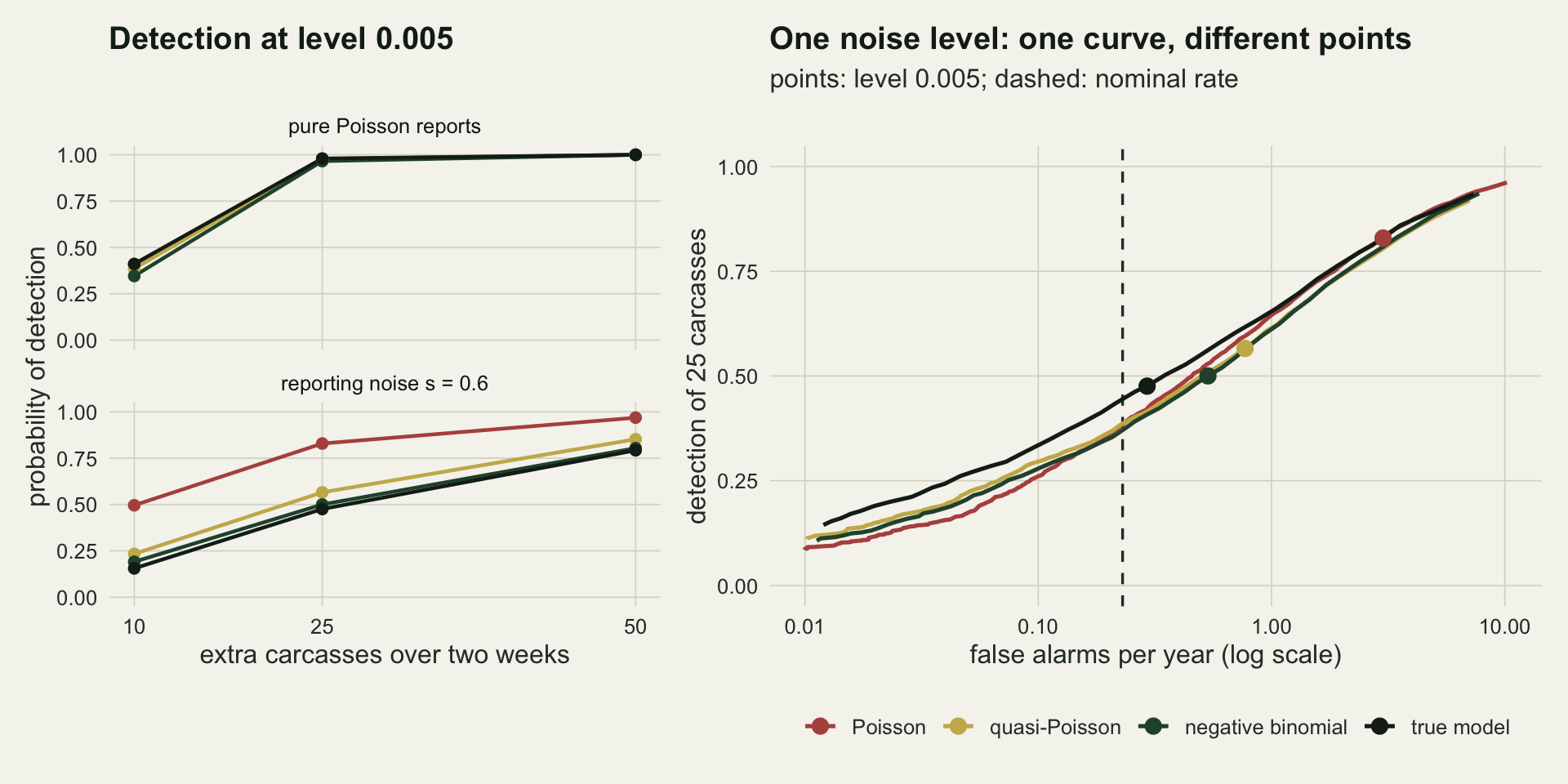
When the noise changes with the season
The near-identical curves have a reason. In the simulation above the reporting noise is the same in every week and the mean moves only by a factor of three, so the true variance of a week follows its mean closely, and a Poisson limit at a stricter level draws almost the same threshold as a negative binomial one. The estimated dispersion then has little to tell the limit that a different level would not. Real reporting is not that even: effort in a holiday month or during a spring bird flu scare swings far more than in a dull November. The next chunk keeps the alarm and the die-off exactly as before and changes only the background, in three arms. The first is the flat control from above, with s = 0.6 and a mean of six every week. In the second the mean stays at six and the noise follows the season, s = 0.6 + 0.45 sin(2 pi w / 52), from 0.15 in autumn to 1.05 in spring. In the third the noise stays at 0.6 and the mean follows the season from two to twenty, so the dispersion, which grows with the mean, differs widely between weeks. These settings were fixed before the run.
roc_of <- function(cell, D = "25") {
  do.call(rbind, lapply(rule_names, function(r) {
    data.frame(rule = r, a = a_grid,
               fa = sapply(a_grid, function(a) fa_rate(cell$p_null[[r]], a)),
               det = sapply(a_grid, function(a) det_rate(cell$p_die[[D]][[r]], a)))
  }))
}
s_season  <- 0.6 + 0.45 * sin(2 * pi * wk_all / 52)
mu_season <- 11 + 9 * sin(2 * pi * wk_all / 52)
set.seed(5505)
cell_snoise <- run_cell(n_rep, s_use, s_week = s_season, mu_week = rep(6, 52),
                        D_set = 25)
set.seed(5506)
cell_wide <- run_cell(n_rep, s_use, mu_week = mu_season, D_set = 25)

arm_names <- c("constant noise, flat mean",
               "seasonal noise, flat mean",
               "constant noise, wide seasonal mean")
arm_cells <- list(flat_cell, cell_snoise, cell_wide)
arm_roc <- lapply(arm_cells, roc_of)
arm_tab <- do.call(rbind, lapply(1:3, function(i) {
  data.frame(arm = arm_names[i], rule = rule_names,
             fa005 = sapply(arm_cells[[i]]$p_null, fa_rate),
             det005 = sapply(arm_cells[[i]]$p_die[["25"]], det_rate),
             det_nom = sapply(rule_names, det_matched, target = fa_nominal,
                              roc = arm_roc[[i]]),
             det_one = sapply(rule_names, det_matched, target = 1,
                              roc = arm_roc[[i]]))
}))
arm_at <- function(i, r, col) arm_tab[arm_tab$arm == arm_names[i] & arm_tab$rule == r, col]
pois_mult_arm <- range(arm_tab$fa005[arm_tab$rule == "Poisson"]) / fa_nominal
nb_mult_arm   <- range(arm_tab$fa005[arm_tab$rule == "negative binomial"]) / fa_nominal
nb_at_pois2 <- det_matched("negative binomial", arm_at(2, "Poisson", "fa005"),
                           roc = arm_roc[[2]])

# seasonal noise arm: detection by the noise at the die-off's first week,
# each rule at the swept level whose false alarm rate is nearest nominal
quiet_die <- s_season[test_wk[cell_snoise$onset]] < s_use
season_split <- sapply(c("Poisson", "negative binomial"), function(r) {
  roc_r <- arm_roc[[2]][arm_roc[[2]]$rule == r & arm_roc[[2]]$fa > 0, ]
  a_r <- roc_r$a[which.min(abs(log(roc_r$fa) - log(fa_nominal)))]
  hit <- cell_snoise$p_die[["25"]][[r]][, "either"] <= a_r
  c(quiet = mean(hit[quiet_die]), noisy = mean(hit[!quiet_die]))
})
At the nominal 0.23 false alarms a year, with each rule’s level set to hit that rate, the Poisson, quasi-Poisson and negative binomial rules and the true model detect a 25-carcass die-off with these probabilities. On the flat control: 0.38, 0.33, 0.32 and 0.38. With the seasonal noise: 0.14, 0.40, 0.43 and 0.50. With the wide seasonal mean: 0.18, 0.28, 0.27 and 0.33.
On the flat control the Poisson rule is not worse than the negative binomial at a matched rate; it detects more. With the noise the same in every week and the mean flat, the dispersion estimate only adds noise to the limit. In the seasonal noise arm the order reverses and the gap is large. The Poisson limit is nearly the same in every week, so to keep its rate down it has to be set high enough for the noisy spring weeks, and it then misses die-offs in the quiet autumn weeks that the negative binomial limit, which estimates the dispersion from each week’s own seven-week window, picks up. Splitting the die-offs by the noise in their first week, each rule at the swept level nearest the nominal rate, the Poisson rule detects 0.05 of those starting in the quieter half of the year and 0.23 in the noisier half; the negative binomial rule 0.66 and 0.20. The wide mean arm lies between the two, and there the Poisson rule loses because the margin of its limit above the mean grows with the square root of the mean while the spread of the counts grows faster. The gap narrows at a looser operating point: at one false alarm a year the Poisson and negative binomial rules detect 0.52 and 0.64 with the seasonal noise, and 0.43 and 0.47 with the wide mean. Far up the curve the seasonal-noise Poisson curve crosses the others: at its own rate of 2.76 false alarms a year it detects 0.81, the negative binomial rule at that rate 0.77. A scheme that tolerates several false alarms a year would not see the difference; one that runs at the nominal rate would.
At level 0.005 the three arms give the Poisson rule 3.04, 2.76 and 4.25 false alarms a year and the negative binomial rule 0.55, 0.52 and 0.50, so in every arm the Poisson rule runs at 12 to 18 times the nominal rate and the negative binomial rule at 2.2 to 2.4 times it. What changes between the arms is how well the rules separate a die-off from a noisy week. A dispersion estimated week by week is a cost when the dispersion is the same all year and a gain when it changes widely between weeks, through the reporting noise or through the mean, and the seasonal mean of the main simulation sits close to the point where the two balance.
season_roc <- do.call(rbind, lapply(1:3, function(i) {
  cbind(arm = arm_names[i], arm_roc[[i]])
}))
season_roc$arm  <- factor(season_roc$arm, levels = arm_names)
season_roc$rule <- factor(season_roc$rule, levels = rule_names)
season_pts <- arm_tab
season_pts$arm  <- factor(season_pts$arm, levels = arm_names)
season_pts$rule <- factor(season_pts$rule, levels = rule_names)
p_season <- ggplot(season_roc[season_roc$fa > 0.01 & season_roc$fa < 12, ],
                   aes(fa, det, colour = rule)) +
  geom_vline(xintercept = fa_nominal, linetype = "dashed",
             colour = te_body, linewidth = 0.6) +
  geom_line(linewidth = 0.9) +
  geom_point(data = season_pts, aes(fa005, det005), size = 2.6) +
  facet_wrap(~ arm, nrow = 1) +
  scale_colour_manual(values = rule_cols, name = NULL) +
  scale_x_log10(breaks = c(0.01, 0.1, 1, 10), labels = c("0.01", "0.1", "1", "10")) +
  scale_y_continuous(limits = c(0, 1)) +
  labs(x = "false alarms per year (log scale)", y = "detection of 25 carcasses",
       title = "When the dispersion changes between weeks, the curves separate",
       subtitle = "points: level 0.005; dashed: nominal rate") +
  theme_datasheet() +
  theme(legend.position = "bottom")
p_season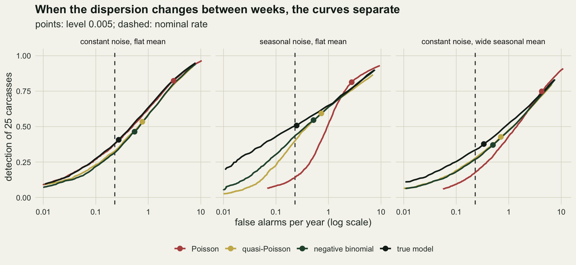
Past die-offs in the baseline, and down-weighting them
A real history is not clean. A die-off five years ago sits in the baseline and inflates both the mean and the dispersion of every window it falls in. Farrington’s algorithm handles this by fitting the baseline, computing Anscombe residuals, and giving every historical week whose residual exceeds one a weight proportional to the inverse square of its residual. Noufaily and colleagues raised that cut-off to 2.58. The next chunk gives each historical year a die-off of 50 carcasses over two weeks with probability one half, and compares the negative binomial limit with no reweighting and with the two cut-offs, on the clean history and on the contaminated one. The current year is clean in the false alarm run, as before.
past_prob <- 0.5
past_D    <- 50
rw_design <- expand.grid(cutoff = c(Inf, 2.58, 1), past = c(0, past_prob))
set.seed(5504)
rw_tab <- do.call(rbind, lapply(seq_len(nrow(rw_design)), function(i) {
  cell <- run_cell(n_rep, s_use, cutoff = rw_design$cutoff[i],
                   past_D = past_D, past_prob = rw_design$past[i], D_set = 25)
  data.frame(cutoff = rw_design$cutoff[i], past = rw_design$past[i],
             fa = fa_rate(cell$p_null[["negative binomial"]]),
             det = det_rate(cell$p_die[["25"]][["negative binomial"]]))
}))
rw_at <- function(cut_v, past_v, col) rw_tab[rw_tab$cutoff == cut_v & rw_tab$past == past_v, col]
rw_tab$curve <- sapply(rw_tab$fa, det_matched, r = "negative binomial")
rw_curve_at <- function(cut_v, past_v) rw_tab$curve[rw_tab$cutoff == cut_v & rw_tab$past == past_v]
On the clean history the negative binomial limit without reweighting gives 0.52 false alarms a year and detects 0.50 of 25-carcass die-offs (a fresh simulation of the cell above). Contaminating the history drops both, to 0.39 and 0.38: the past die-offs raise the limit.
Reweighting at Farrington’s cut-off of one on the contaminated history gives 1.04 and 0.60; at 2.58, 0.58 and 0.47. On the clean history, where there is nothing to remove, the cut-off of one still moves the rate to 1.36, and 2.58 to 0.73. With overdispersed reports, a residual above one is ordinary, so the cut-off of one down-weights the upper part of every baseline, pulls the mean and the dispersion down and lowers the limit. It is one of the sources of excess false reports that Noufaily and colleagues addressed, alongside the trend, the seasonality and the error distribution.
The clean negative binomial curve from the detection section gives a yardstick for all six points. Past die-offs push the rule below that curve: at 0.39 false alarms a year the clean curve detects 0.45, the contaminated baseline 0.38. Down-weighting recovers most of that loss (at the cut-off of one, 0.60 against 0.62 on the curve; at 2.58, 0.47 against 0.51) and at the same time moves the rule up the curve to a higher false alarm rate. On the clean history the three points lie on the curve (0.50, 0.56 and 0.68 measured against 0.50, 0.55 and 0.67), so there the reweighting only moves the operating point.
rw_tab$weighting <- factor(ifelse(is.finite(rw_tab$cutoff),
                                  paste("cut-off", rw_tab$cutoff), "no reweighting"),
                           levels = c("no reweighting", "cut-off 2.58", "cut-off 1"))
rw_tab$history <- factor(ifelse(rw_tab$past == 0, "clean history", "past die-offs in history"),
                         levels = c("clean history", "past die-offs in history"))
ggplot(rw_tab, aes(fa, det, colour = weighting, shape = history)) +
  geom_vline(xintercept = fa_nominal, linetype = "dashed",
             colour = te_body, linewidth = 0.6) +
  geom_line(aes(group = history), colour = te_line, linewidth = 0.8) +
  geom_point(size = 3.4) +
  scale_colour_manual(values = c(te_ink, te_gold, te_rust), name = NULL) +
  scale_shape_manual(values = c(16, 17), name = NULL) +
  scale_x_continuous(limits = c(0, NA)) +
  labs(x = "false alarms per year", y = "detection of 25 carcasses",
       title = "Down-weighting repairs a contaminated baseline",
       subtitle = "negative binomial limit; dashed: nominal rate") +
  theme_datasheet() +
  theme(legend.position = "bottom", legend.box = "vertical")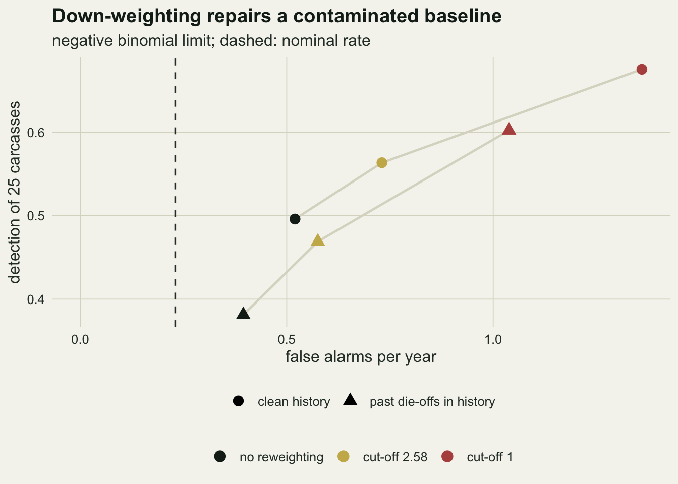
What to report
Report the false alarm rate the scheme actually runs at, measured, not the level typed into the code. For weekly counts it is easiest to simulate from the scheme’s own history: fit the baseline, simulate years from the fitted mean and dispersion (or resample whole historical years), run the alarm, and count. State it per year, and state the share of years with at least one false alarm, because that is the figure the people who answer alarms feel.
Report detection for a stated die-off size, duration and alarm definition, at that measured rate. “Detects a die-off” means nothing without the number of extra carcasses, the number of weeks and whether an alarm in any week counts. A detection figure quoted from a rule that over-alarms is a point higher up the curve, not a better rule.
Report the dispersion estimate and how many historical weeks it came from, and check whether the reporting noise is the same through the year: compare the dispersion of the baseline windows between seasons. A dispersion from thirty five weeks has a wide spread. If the dispersion is about the same all year, a stricter level on a simpler limit does about as well as a different distribution. If it changes between seasons, the level cannot stand in for the variance model: a limit that follows the week’s own dispersion finds die-offs in the quiet season that a single strict limit misses.
If past die-offs are down-weighted, report the cut-off and check the rate on a clean stretch of history: at a cut-off of one the reweighting itself raised the false alarm rate on a history with nothing to remove.
Honest limits
The reporting noise is independent from week to week. Real reporting effort is autocorrelated: a news story about dead birds raises reports for several weeks, and a wet month lowers them for a month. Autocorrelated noise makes the current week look more like its neighbours, which a baseline built from other years does not know about, so both the false alarm rate and the chance that a reporting surge is read as a die-off would be higher than here.
The die-off adds carcasses to a scheme whose reporting effort does not react. In a real scheme the first reports of a die-off bring publicity and more reporting, which helps detection in the second week and would make the first-week share lower than the figures above.
The baseline has no trend and the simulation fits none. Farrington’s algorithm fits a log-linear trend across the years and keeps it only when it is significant; with a growing reporting scheme, as many citizen reporting schemes are, the trend term is a further estimated quantity from the same thirty five weeks and its own source of false alarms. Noufaily and colleagues also changed how the trend and the seasonality are handled, and none of that is implemented here. The limits here are one-sided at level 0.005 per week, while the surveillance package’s implementation of the original algorithm takes the normal quantile at one minus half its level, so its nominal rates are not directly comparable with the numbers here.
Only historical-limits alarms are compared. CUSUM-type and other sequential methods accumulate evidence over several weeks and, for a die-off spread over a fortnight, may detect at a lower false alarm cost; Unkel and colleagues review them. Many schemes also rely on a person reading the reports, which no simulation of counts captures: a single report of forty dead geese at one lake is a die-off to a reader and one entry to a weekly total if it is logged as one report.
Detection is judged per event, with a fixed two-week die-off at a random tested week. A delay distribution over longer die-offs, or a die-off concentrated in one week, would change the level of every curve, and the comparison between rules would need to be redone at those settings. The finding that the rules share nearly one curve holds only when the reporting noise is the same in every week and the mean varies modestly; it was measured for the 25-carcass, two-week die-off at s = 0.6, and the seasonal arms show that it breaks when the dispersion differs widely between weeks. Those arms use one shape of seasonal change each, in phase with the tested weeks; a noise that changes abruptly (a news story) rather than smoothly would be caught less well by a seven-week window.
References
Farrington CP, Andrews NJ, Beale AD, Catchpole MA 1996 Journal of the Royal Statistical Society Series A 159(3):547-563 (10.2307/2983331)
Noufaily A, Enki DG, Farrington P, Garthwaite P, Andrews N, Charlett A 2013 Statistics in Medicine 32(7):1206-1222 (10.1002/sim.5595)
Unkel S, Farrington CP, Garthwaite PH, Robertson C, Andrews N 2012 Journal of the Royal Statistical Society Series A 175(1):49-82 (10.1111/j.1467-985X.2011.00714.x)