library(ggplot2)

te_paper  <- "#f5f4ee"
te_ink    <- "#16241d"
te_body   <- "#2c3a31"
te_forest <- "#275139"
te_rust   <- "#b5534e"
te_gold   <- "#c9b458"
te_line   <- "#dad9ca"

theme_datasheet <- function() {
  theme_minimal(base_size = 12) +
    theme(plot.background  = element_rect(fill = te_paper, colour = NA),
          panel.background = element_rect(fill = te_paper, colour = NA),
          panel.grid.major = element_line(colour = te_line, linewidth = 0.3),
          panel.grid.minor = element_blank(),
          text             = element_text(colour = te_body),
          plot.title       = element_text(colour = te_ink, face = "bold"),
          plot.subtitle    = element_text(colour = te_body),
          axis.text        = element_text(colour = te_body))
}Reference sites and tolerance bounds
R
bioassessment
monitoring
statistics
simulation
ecology tutorial
Tolerance bounds versus percentiles for impairment thresholds from reference sites in R: the false alarm guarantee, its cost in power, and skewed indices.
A regional survey has sampled twelve streams that everyone agrees are in good condition, and has scored each one on a stream condition index. The next task is the one the survey was paid for: a rule that says when a stream elsewhere in the region is scoring low enough to be called impaired. The obvious rule takes the lowest five per cent of the reference scores as the boundary. A stream that falls below the fifth percentile of twelve good streams is flagged, and the implied promise is that a good stream would be flagged only one time in twenty.
That promise is about a quantity nobody observes. The true fifth percentile belongs to the population of all good streams in the region, and twelve streams estimate it with a great deal of noise. Some reference sets put the boundary too high and will flag far more than one good stream in twenty; others put it too low. A tolerance bound is the statistical object built for exactly this: a threshold computed from the sample so that, with a stated confidence, at most a stated share of the reference population falls below it. The post measures what that confidence buys and what it costs, and then shows it failing on the two kinds of skew that biotic indices actually have.
The guarantee here is of a different kind from the one in conformal prediction intervals from scratch. There, “The guarantee holds” repeats the whole procedure over fresh data and counts coverage averaged over calibration sets and test points together, and “Marginal is not conditional” is about conditioning on the covariate. A tolerance bound makes a promise about the false alarm rate of the threshold from each calibration set: at most five per cent, for all but five per cent of reference sets. Averaged coverage, the quantity checked in checking predictive calibration and coverage under “Does the interval cover what it claims?”, can be right on target while a large share of individual reference sets are badly wrong. Restoration trajectories and recovery treats reference sites as a moving target under “The reference moves” and sets no threshold rule; here the reference population holds still and the rule is the whole subject. The power calculations are a special case of power analysis by simulation, with the threshold rule in place of a model.
Nothing below claims that any agency uses a 95/95 tolerance bound. Bioassessment programmes more often use a percentile of the reference distribution or a ratio of observed to expected taxa, as Stoddard and colleagues and Hawkins and colleagues describe. What is simulated is a set of threshold rules applied to reference samples from known distributions, so that the true false alarm rate of each threshold can be computed exactly.
One reference set, two thresholds
The rules compared throughout are fixed here, before any simulation. The target share is five per cent and the confidence is ninety five per cent. The empirical fifth percentile uses R’s default quantile, type 7 in the Hyndman and Fan numbering, which interpolates between two adjacent order statistics. The normal fifth percentile is the mean minus 1.645 standard deviations. The one-sided 95/95 normal tolerance bound is the mean minus k standard deviations, where k comes from the noncentral t distribution, as in Krishnamoorthy and Mathew. The minimum of the reference set is the order statistic rule.
p_share <- 0.05                                 # share of good sites allowed below
g_conf  <- 0.95                                 # confidence of the tolerance bound
z_p     <- qnorm(1 - p_share)

k_tol <- function(n) {
  # pnt warns about precision at the largest n; the simulated rows check k
  suppressWarnings(qt(g_conf, n - 1, ncp = z_p * sqrt(n)) / sqrt(n))
}
row_sd <- function(m) sqrt(rowSums((m - rowMeans(m))^2) / (ncol(m) - 1))
row_q7 <- function(m, p = p_share) {
  srt <- t(apply(m, 1, sort))
  h   <- (ncol(m) - 1) * p + 1
  lo  <- floor(h)
  srt[, lo] + (h - lo) * (srt[, lo + 1] - srt[, lo])
}
thresholds <- function(m) {
  mu_r <- rowMeans(m); sd_r <- row_sd(m)
  cbind(empirical = row_q7(m),
        normal    = mu_r - z_p * sd_r,
        tolerance = mu_r - k_tol(ncol(m)) * sd_r,
        minimum   = apply(m, 1, min))
}

n_ex    <- 12
idx_mu  <- 70                                   # index mean in good streams
idx_sd  <- 8                                    # index sd in good streams
set.seed(1207)
ref_ex  <- matrix(rnorm(n_ex, idx_mu, idx_sd), nrow = 1)
thr_ex  <- thresholds(ref_ex)[1, ]
q7_chk  <- abs(thr_ex[["empirical"]] - quantile(ref_ex[1, ], p_share))
site_ex <- (thr_ex[["empirical"]] + thr_ex[["tolerance"]]) / 2
fa_ex   <- pnorm(thr_ex, idx_mu, idx_sd)
k_ex    <- k_tol(n_ex)
The twelve reference streams have index scores with a mean of 67.9 and a standard deviation of 5.9, drawn from a population of good streams with mean 70 and standard deviation 8. The empirical fifth percentile is 58.9 (the hand-rolled interpolation agrees with quantile() to 0.0e+00). With twelve sites the tolerance factor is 2.736 rather than 1.645, and the tolerance bound is 51.7.
A test stream scoring 55.3, halfway between the two, is impaired under the percentile rule and in good condition under the tolerance bound. Because the reference population is known here, the true false alarm rate of each threshold can be read straight off the normal distribution function: the empirical percentile from this set would flag 8.3 per cent of good streams, and the tolerance bound 1.10 per cent. In the field neither number is available, which is why the question has to be asked over many reference sets.
The false alarm rate belongs to the reference set
For a single reference set, the true false alarm rate of a threshold is the reference distribution function evaluated at the threshold. That is exact, so each simulated reference set contributes one exact rate, and no second layer of Monte Carlo is needed to score it. The quantity a tolerance bound controls is the share of reference sets whose rate exceeds five per cent.
The impaired site is the reference population shifted down by two standard deviations. Power is the probability that such a site falls below the threshold, again read from the distribution function for each reference set and averaged.
n_grid <- c(10, 20, 30, 50, 100)
n_rep  <- 4000
shift  <- 2                                     # impairment in reference sds
mcse_p <- sqrt(p_share * (1 - p_share) / n_rep)

set.seed(3101)
fa_keep <- list()
norm_tab <- do.call(rbind, lapply(n_grid, function(n) {
  thr <- thresholds(matrix(rnorm(n_rep * n), ncol = n))
  fa  <- pnorm(thr)
  pw  <- pnorm(thr + shift)
  if (n %in% c(10, 50)) fa_keep[[as.character(n)]] <<- fa
  data.frame(n = n, rule = colnames(thr), mean_fa = colMeans(fa),
             p_over = colMeans(fa > p_share), power = colMeans(pw))
}))

# closed forms for the normal rows
over_closed <- function(n, fac) 1 - pt(fac * sqrt(n), n - 1, ncp = z_p * sqrt(n))
closed_tab <- data.frame(
  n         = n_grid,
  normal    = sapply(n_grid, function(n) over_closed(n, z_p)),
  tolerance = sapply(n_grid, function(n) suppressWarnings(over_closed(n, k_tol(n)))),
  minimum   = (1 - p_share)^n_grid,
  emp_lo    = sapply(n_grid, function(n) {
    lo <- floor((n - 1) * p_share + 1)
    pbeta(p_share, lo, n - lo + 1, lower.tail = FALSE) }),
  emp_hi    = sapply(n_grid, function(n) {
    lo <- floor((n - 1) * p_share + 1)
    pbeta(p_share, lo + 1, n - lo, lower.tail = FALSE) }))

get_v <- function(tab, nn, rr, col) tab[tab$n == nn & tab$rule == rr, col]
sim_long <- norm_tab[norm_tab$rule %in% c("normal", "tolerance", "minimum"), ]
closed_v <- mapply(function(nn, rr) closed_tab[closed_tab$n == nn, rr],
                   sim_long$n, as.character(sim_long$rule))
gap_se   <- max(abs(sim_long$p_over - closed_v) /
                sqrt(closed_v * (1 - closed_v) / n_rep))
emp_in   <- all(norm_tab$p_over[norm_tab$rule == "empirical"] >= closed_tab$emp_lo - 3 * mcse_p &
                norm_tab$p_over[norm_tab$rule == "empirical"] <= closed_tab$emp_hi + 3 * mcse_p)
Each cell uses 4000 reference sets, fixed before the run, so a share near five per cent carries a Monte Carlo standard error of 0.0034.
Start with ten reference sites. The empirical fifth percentile gives an average false alarm rate of 0.121, and 77.1 per cent of reference sets produce a threshold whose own false alarm rate is above five per cent. The normal fifth percentile does better on average, 0.076, and still exceeds five per cent in 55.0 per cent of sets. The tolerance bound exceeds it in 5.2 per cent, which is its nominal five, and its average false alarm rate is 0.011.
More sites do not rescue the percentile rules on this measure. At fifty sites the empirical percentile still exceeds five per cent in 64.6 per cent of sets and the normal percentile in 51.4 per cent. That is not a failure of estimation: both thresholds converge on the true fifth percentile, and a threshold that is centred on the target lands above it in roughly half of all sets (the empirical percentile is also biased upwards at these sizes, with a mean false alarm rate of 0.067 at fifty sites). Only the rules that deliberately stand back from the estimate keep the share of bad sets small.
The simulated rows are an integrator check against closed forms, not a finding. The share of sets above five per cent for the normal percentile and the tolerance bound follows from the noncentral t distribution of the standardised mean, and for the minimum it is exactly 0.95 to the power n. Across the fifteen normal, tolerance and minimum cells the largest disagreement is 2.3 binomial standard errors. The type 7 empirical percentile is an interpolation between two order statistics, so it has no single Beta form; its simulated share lies between the Beta tail probabilities of the two bracketing order statistics in every cell (checked).
fa_df <- do.call(rbind, lapply(names(fa_keep), function(nm) {
  fa <- fa_keep[[nm]][, c("empirical", "normal", "tolerance")]
  data.frame(sites = paste(nm, "sites"),
             rule = rep(c("empirical 5th pct", "mean - 1.645 sd",
                          "95/95 tolerance"), each = nrow(fa)),
             fa = as.vector(fa))
}))
fa_df$rule  <- factor(fa_df$rule, levels = c("empirical 5th pct",
                                              "mean - 1.645 sd", "95/95 tolerance"))
fa_df$sites <- factor(fa_df$sites, levels = c("10 sites", "50 sites"))

ggplot(fa_df, aes(fa)) +
  geom_histogram(aes(fill = rule), binwidth = 0.01, boundary = 0, colour = NA) +
  geom_vline(xintercept = p_share, linetype = "dashed", colour = te_ink, linewidth = 0.6) +
  facet_grid(sites ~ rule) +
  scale_fill_manual(values = c(te_gold, te_rust, te_forest), guide = "none") +
  coord_cartesian(xlim = c(0, 0.3)) +
  scale_x_continuous(breaks = c(0, 0.1, 0.2)) +
  labs(x = "true false alarm rate of the threshold", y = "reference sets",
       title = "Five per cent, reference set by reference set",
       subtitle = "dashed line: the five per cent the rule is meant to deliver") +
  theme_datasheet() +
  theme(strip.text = element_text(colour = te_ink))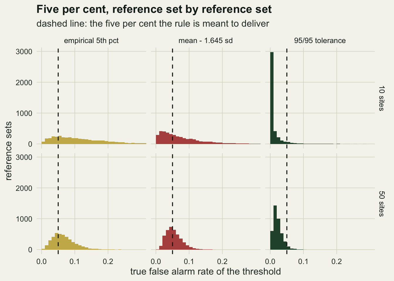
The guarantee is paid for in power
A threshold that sits further down flags fewer good streams and fewer impaired ones. The price of the tolerance bound is paid in the second currency.
pow_emp10 <- get_v(norm_tab, 10, "empirical", "power")
pow_tol10 <- get_v(norm_tab, 10, "tolerance", "power")
pow_emp50 <- get_v(norm_tab, 50, "empirical", "power")
pow_tol50 <- get_v(norm_tab, 50, "tolerance", "power")
pow_tol100 <- get_v(norm_tab, 100, "tolerance", "power")
pow_nrm100 <- get_v(norm_tab, 100, "normal", "power")
pow_ideal <- pnorm(-z_p + shift)
pow_min10  <- get_v(norm_tab, 10, "minimum", "power")
pow_min100 <- get_v(norm_tab, 100, "minimum", "power")
mcse_pow   <- sqrt(0.25 / n_rep)
With the true fifth percentile known, a site two standard deviations down would be flagged with probability 0.639. At ten reference sites the empirical percentile reaches 0.738 and the tolerance bound 0.255. The percentile’s power exceeds the ideal for the same reason its false alarm rate does: a threshold that is too high flags everything more often. At fifty sites the pair is 0.667 against 0.477, and at a hundred the tolerance bound reaches 0.531 against 0.639 for the normal percentile. The Monte Carlo standard error of any power here is at most 0.0079.
The gap closes only because k shrinks towards 1.645 as sites are added, and it shrinks slowly. The minimum goes the other way: its threshold falls as the set grows, and its power drops from 0.657 at ten sites to 0.322 at a hundred.
pow_df <- norm_tab
pow_df$rule <- factor(pow_df$rule, levels = c("empirical", "normal", "tolerance", "minimum"),
                      labels = c("empirical 5th percentile", "mean - 1.645 sd",
                                 "95/95 tolerance bound", "minimum"))
ggplot(pow_df, aes(n, power, colour = rule)) +
  geom_hline(yintercept = pow_ideal, linetype = "dashed", colour = te_body, linewidth = 0.6) +
  geom_line(linewidth = 0.9) +
  geom_point(size = 2.2) +
  scale_x_log10(breaks = n_grid) +
  scale_colour_manual(values = c(te_gold, te_rust, te_forest, te_ink), name = NULL) +
  scale_y_continuous(limits = c(0, 1)) +
  labs(x = "reference sites (log scale)", y = "power at a two sd impairment",
       title = "Only more sites pay for the guarantee",
       subtitle = "dashed line: power with the true fifth percentile known") +
  theme_datasheet() +
  theme(legend.position = "bottom") +
  guides(colour = guide_legend(nrow = 2))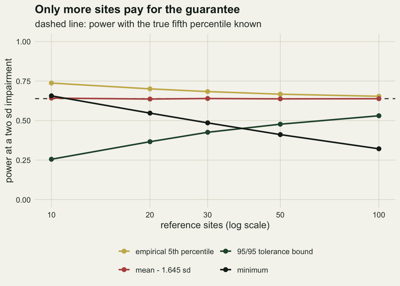
A left-skewed index breaks the guarantee, and more sites break it further
The noncentral t argument needs the reference scores to be normal. Many biotic indices are shares bounded above by one, and good sites pile up near the top with a long tail towards lower values. A beta distribution with shape parameters 8 and 2 has that shape, and a beta with shape parameters 4 and 1 is a second, more strongly left-skewed choice used as a check. The impairment is again additive, two reference standard deviations down, because the index is a share and a loss of sensitive taxa subtracts from it.
A right-skewed metric behaves differently. A lognormal with log standard deviation 0.6 stands in for a positive quantity such as a density or a biomass. For that metric the impairment is multiplicative, the site value times exp(-2 x 0.6), which is two standard deviations on the log scale: a density that falls by a constant factor is the natural damage model for a positive quantity, and an additive shift of two raw standard deviations would push most impaired values below zero. The additive version is carried along as a sensitivity line. For the lognormal a fifth rule is added, the same tolerance bound computed on log values and back-transformed.
sdlog_use <- 0.6
beta_sd   <- function(a, b) sqrt(a * b / ((a + b)^2 * (a + b + 1)))
beta_skew <- function(a, b) 2 * (b - a) * sqrt(a + b + 1) / ((a + b + 2) * sqrt(a * b))
skew_b82  <- beta_skew(8, 2)
skew_b41  <- beta_skew(4, 1)
skew_set <- list(
  "beta(8, 2)"   = list(r = function(m) rbeta(m, 8, 2),   p = function(q) pbeta(q, 8, 2),
                        sd = beta_sd(8, 2)),
  "beta(4, 1)" = list(r = function(m) rbeta(m, 4, 1), p = function(q) pbeta(q, 4, 1),
                        sd = beta_sd(4, 1)),
  "lognormal"    = list(r = function(m) rlnorm(m, 0, sdlog_use),
                        p = function(q) plnorm(q, 0, sdlog_use),
                        sd = sqrt((exp(sdlog_use^2) - 1) * exp(sdlog_use^2))))

set.seed(3102)
skew_tab <- do.call(rbind, lapply(names(skew_set), function(dn) {
  dd <- skew_set[[dn]]
  do.call(rbind, lapply(n_grid, function(n) {
    x_m <- matrix(dd$r(n_rep * n), ncol = n)
    thr <- thresholds(x_m)
    log_m <- log(x_m)
    thr <- cbind(thr, log_tolerance = exp(rowMeans(log_m) - k_tol(n) * row_sd(log_m)))
    fa  <- dd$p(thr)
    pw_add <- dd$p(thr + shift * dd$sd)
    pw  <- if (dn == "lognormal") dd$p(thr * exp(shift * sdlog_use)) else pw_add
    data.frame(dist = dn, n = n, rule = colnames(thr), mean_fa = colMeans(fa),
               p_over = colMeans(fa > p_share), power = colMeans(pw),
               power_add = colMeans(pw_add), below_zero = colMeans(thr <= 0))
  }))
}))
gs <- function(dn, nn, rr, col) skew_tab[skew_tab$dist == dn & skew_tab$n == nn &
                                         skew_tab$rule == rr, col]
b82  <- skew_tab[skew_tab$dist == "beta(8, 2)" & skew_tab$rule == "tolerance", ]
b41 <- skew_tab[skew_tab$dist == "beta(4, 1)" & skew_tab$rule == "tolerance", ]
q05_b82  <- qbeta(p_share, 8, 2)
nq05_b82 <- 0.8 - z_p * beta_sd(8, 2)
imp_neg <- plnorm(shift * skew_set$lognormal$sd, 0, sdlog_use)
On beta(8, 2) the raw tolerance bound exceeds a five per cent false alarm rate in 17.0 per cent of reference sets at ten sites, against a nominal five with a Monte Carlo standard error under a percentage point. The share rises with every step in n: 22.2, 24.6, 32.5 and 47.2 per cent at 20, 30, 50 and 100 sites. The second left-skewed choice, with moment skewness -1.05 against -0.83 for beta(8, 2), repeats the rise with n, from 24.2 per cent at ten sites to 63.6 per cent at a hundred.
The mechanism is that the normal model gets the lower tail wrong in a fixed direction. A left-skewed population has a fifth percentile lower than the mean minus 1.645 standard deviations would suggest: for beta(8, 2) the true fifth percentile is 0.571, while the population mean minus 1.645 population standard deviations is 0.602. The normal fit places the target too high. At ten sites the tolerance factor is large enough to cover that error most of the time; as sites are added, k falls towards 1.645 and the margin that was hiding the misfit disappears, while the bias itself does not shrink. The bound converges, confidently, on the wrong value. Taking logs does not help a left-skewed share: the log-scale bound exceeds five per cent in 55.5 per cent of beta(8, 2) sets at a hundred sites, because a log makes a left skew stronger.
The lognormal fails in the opposite direction. The raw tolerance bound lies at or below zero in 95.8 per cent of reference sets at ten sites and 98.0 per cent at a hundred. A positive metric can never fall below a negative threshold, so under the multiplicative impairment the raw bound has power 0.007 at ten sites and 0.000 at a hundred. Its false alarm guarantee holds, trivially, because it flags nothing. Computed on the log scale, where the lognormal is normal, the same bound is exact again: 4.9 per cent of sets above five per cent at ten sites and 4.5 per cent at a hundred, with power 0.249 rising to 0.529.
The lognormal power result depends on the damage model, and the sensitivity line shows how much. With an additive impairment of two raw standard deviations, the raw tolerance bound has power 0.359 at ten sites and the log-scale bound 0.829. Those numbers are inflated by an impossible quantity: an additive shift of that size sends 77.6 per cent of impaired values below zero, and every one of them falls below any non-negative threshold such as the log-scale bound. The raw bound is itself negative in most sets, so it flags far fewer of them. The conclusion that survives both damage models is the false alarm one; the power ordering between raw and log scales holds under both, but its size does not.
over_df <- rbind(
  data.frame(dist = "normal", n = n_grid, rule = "raw tolerance bound",
             p_over = norm_tab$p_over[norm_tab$rule == "tolerance"]),
  data.frame(dist = "normal", n = n_grid, rule = "minimum",
             p_over = norm_tab$p_over[norm_tab$rule == "minimum"]),
  do.call(rbind, lapply(names(skew_set), function(dn) {
    sub_rows <- skew_tab[skew_tab$dist == dn & skew_tab$rule %in% c("tolerance", "log_tolerance", "minimum"), ]
    data.frame(dist = dn, n = sub_rows$n,
               rule = c(tolerance = "raw tolerance bound", log_tolerance = "log-scale tolerance bound",
                        minimum = "minimum")[as.character(sub_rows$rule)],
               p_over = sub_rows$p_over)
  })))
over_df$dist <- factor(over_df$dist, levels = c("normal", "beta(8, 2)", "beta(4, 1)", "lognormal"))
over_df$rule <- factor(over_df$rule, levels = c("raw tolerance bound", "log-scale tolerance bound", "minimum"))

ggplot(over_df, aes(n, p_over, colour = rule)) +
  geom_hline(yintercept = p_share, linetype = "dashed", colour = te_body, linewidth = 0.6) +
  geom_line(linewidth = 0.9) +
  geom_point(size = 2) +
  facet_wrap(~ dist, nrow = 1) +
  scale_x_log10(breaks = c(10, 30, 100), expand = expansion(mult = 0.08)) +
  scale_colour_manual(values = c(te_forest, te_gold, te_ink), name = NULL) +
  labs(x = "reference sites (log scale)", y = "share of sets with false alarm above 5%",
       title = "The normal-theory promise, off the normal",
       subtitle = "dashed line: the five per cent a 95/95 bound promises") +
  theme_datasheet() +
  theme(legend.position = "bottom", strip.text = element_text(colour = te_ink),
        panel.spacing.x = unit(1.4, "lines"))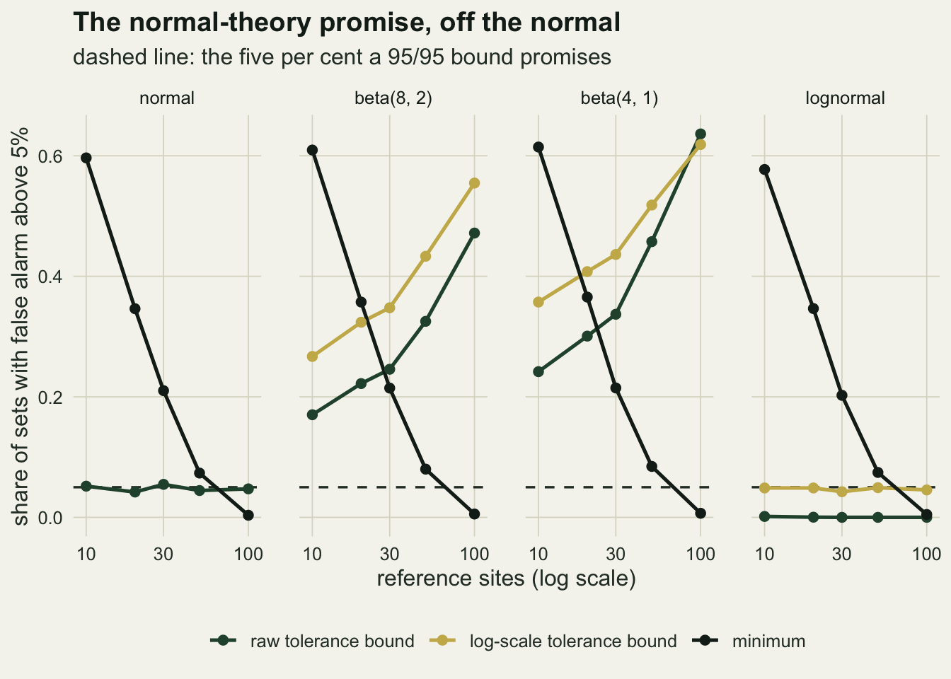
The order-statistic rule needs fifty nine sites
There is one threshold whose guarantee does not depend on the shape of the reference distribution. The distribution function evaluated at the smallest of n reference values has a Beta(1, n) distribution for any continuous population, so the chance that the minimum sits above the true fifth percentile is exactly 0.95 to the power n. Wilks worked out sample sizes for such distribution-free tolerance limits in 1941.
n_wilks <- ceiling(log(1 - g_conf) / log(1 - p_share))
# smallest n at which the second smallest value reaches the same confidence
n_second <- min(which(pbinom(1, 1:500, p_share, lower.tail = FALSE) >= g_conf))
conf_min <- 1 - (1 - p_share)^c(10, 20, 30, 50, n_wilks, 100)
set.seed(3103)
min_chk <- sapply(skew_set, function(dd) {
  x_m <- matrix(dd$r(n_rep * n_wilks), ncol = n_wilks)
  mean(dd$p(apply(x_m, 1, min)) > p_share)
})
min_chk <- c(normal = mean(pnorm(apply(matrix(rnorm(n_rep * n_wilks), ncol = n_wilks), 1, min)) > p_share),
             min_chk)
min_z <- max(abs(min_chk - (1 - conf_min[5])) / sqrt(conf_min[5] * (1 - conf_min[5]) / n_rep))
pow_min_b82  <- gs("beta(8, 2)", 100, "minimum", "power")
pow_tol_b82  <- gs("beta(8, 2)", 100, "tolerance", "power")
The confidence that the minimum lies at or below the true fifth percentile is 0.401 at ten sites, 0.923 at fifty, and reaches ninety five per cent only at 59 sites (0.952). Simulated at that size, the share of sets above five per cent is 0.0465, 0.0505, 0.0542, 0.0517 for the normal, beta(8, 2), beta(4, 1) and lognormal populations, against the exact 0.0485, the largest gap being 1.7 binomial standard errors. Here the target really is the same number for all four populations, because the rule only looks at ranks.
The cost is the one already seen in the power figure. At a hundred beta(8, 2) reference sites the minimum flags a two standard deviation impairment with power 0.172, against 0.471 for the raw tolerance bound that has lost its guarantee. Below fifty nine sites the minimum does not deliver ninety five per cent confidence at all, and above it the threshold keeps falling as more extreme good sites are found.
What to report
State what the threshold promises and over what. “Five per cent false alarm” said of a percentile is at best an average over reference sets that were never drawn, and at ten sites not even that (the empirical percentile averaged 0.121); said of a tolerance bound it is a statement about the one set in hand, with a confidence attached. The difference is the difference between the left and right columns of the first figure, and a reader cannot recover it from the threshold value.
Report the number of reference sites next to the threshold, and the factor used. A tolerance factor of 2.911 at ten sites and 1.927 at a hundred tells a reader directly how much power was spent on the guarantee.
Look at the shape of the reference scores before choosing the scale. A share with a long lower tail makes a normal-theory bound optimistic, and in the simulations more reference sites made that worse, not better. A positive metric with a right skew needs the bound on the log scale, or the raw bound can be a negative number that never flags anything. If the shape cannot be trusted and the set is large enough, the minimum of at least 59 sites is the rule whose promise holds for any continuous population.
Say how impairment was defined when quoting power. For a positive metric, additive and multiplicative damage give different power figures from identical thresholds.
Honest limits
The reference populations here are known, stable and independent. Real reference sites are chosen by judgement, are spatially correlated, and carry natural gradients that a single distribution ignores; programmes that model expected condition from site covariates, as the O/E approach described by Hawkins and colleagues does, are addressing a harder problem than the one simulated.
The skew results cover three distributions. They show that the normal-theory guarantee fails on left-skewed shares and that the failure grows with sample size for those two beta shapes, at skewness -0.83 and -1.05; they do not give a correction, and a mildly skewed index would sit somewhere between the normal and beta rows. A transformation matched to the shape (a logit for a share, for instance) was not tested.
A threshold is applied here to a single score from a single visit. A test site is itself measured with error, and a programme that averages repeated visits or samples changes both the false alarm rate and the power in ways these numbers do not include.
The impairment is a clean shift of the whole distribution by two standard deviations. Real degradation often changes the spread as well as the location, and a two standard deviation shift is a large effect; smaller shifts give lower power for every rule, and the power gaps quoted above were measured at two standard deviations only.
The nonparametric rule shown is the minimum only. From 93 sites the second smallest value carries the same confidence with better power, and the Beta distribution gives its guarantee in the same way; that refinement was not simulated.
References
Wilks SS 1941 The Annals of Mathematical Statistics 12(1):91-96 (10.1214/aoms/1177731788)
Hyndman RJ, Fan Y 1996 The American Statistician 50(4):361-365 (10.1080/00031305.1996.10473566)
Krishnamoorthy K, Mathew T 2009 Statistical Tolerance Regions: Theory, Applications, and Computation (ISBN 978-0-470-38026-0)
Stoddard JL, Larsen DP, Hawkins CP, Johnson RK, Norris RH 2006 Ecological Applications 16(4):1267-1276 (10.1890/1051-0761(2006)016[1267:SEFTEC]2.0.CO;2)
Hawkins CP, Olson JR, Hill RA 2010 Journal of the North American Benthological Society 29(1):312-343 (10.1899/09-092.1)