library(ggplot2)

te_paper  <- "#f5f4ee"
te_ink    <- "#16241d"
te_body   <- "#2c3a31"
te_forest <- "#275139"
te_rust   <- "#b5534e"
te_gold   <- "#c9b458"
te_line   <- "#dad9ca"

theme_datasheet <- function() {
  theme_minimal(base_size = 12) +
    theme(plot.background  = element_rect(fill = te_paper, colour = NA),
          panel.background = element_rect(fill = te_paper, colour = NA),
          panel.grid.major = element_line(colour = te_line, linewidth = 0.3),
          panel.grid.minor = element_blank(),
          text             = element_text(colour = te_body),
          plot.title       = element_text(colour = te_ink, face = "bold"),
          plot.subtitle    = element_text(colour = te_body),
          axis.text        = element_text(colour = te_body),
          strip.text       = element_text(colour = te_ink))
}Carcass searches and fatality estimates
R
mortality
imperfect detection
simulation
ecology tutorial
Fatality totals from carcass searches depend on whether missed carcasses stay findable. Shoenfeld and Huso bracket the truth when persistence is right, in R.
A wind farm operator has agreed to a year of fatality monitoring. A field worker walks a square plot under each turbine along fixed transects and records every dead bat and bird. The count is not the answer anyone wants. Scavengers remove carcasses between visits, a carcass in long grass is easy to walk past, and the consenting authority wants the number of animals the turbines killed, not the number somebody happened to find. So the monitoring plan carries two side experiments. Trial carcasses are laid out and checked until they disappear, which measures persistence; other trial carcasses are placed without the searcher knowing where, which measures searcher efficiency. The fatality estimate divides the count by a detection probability g built from those two pieces.
The step that decides g is not in either experiment. A carcass that was present at a search and was missed may still be there at the next search. Whether the searcher has the same chance of finding it again, a smaller chance, or no chance at all is a property of the carcass, the vegetation and the searcher, and a single-search efficiency trial says nothing about it. Following Korner-Nievergelt and colleagues, call the factor by which efficiency is multiplied after each miss k: efficiency p on the first search after death, kp on the second, k squared p on the third. Two published estimators take opposite fixed values of it. Shoenfeld’s estimator (an unpublished 2004 report, in the form given by Huso 2011) adds up every later search at the same efficiency, which is k = 1. Huso’s own estimator counts only the first search after death, which is k = 0, and Huso’s simulations found it biased upward when missed carcasses could be found later.
This site has already treated imperfect detection of live animals. How many visits? Occupancy survey design prices a run of blank visits with the expression 1 - (1 - p)^K, which holds detection fixed across visits: the live-animal version of k = 1. Horvitz-Thompson for adaptive samples weights each observed unit by the inverse of its inclusion probability, and the fatality estimator is the same idea applied to carcasses. Interval-censored survival from visit data tracks radio-tagged birds and lists, among its limits, that every carcass is found on the first visit after death. Here that assumption is the subject.
The post does four things. It computes g exactly for a twelve-week season and checks that the Shoenfeld and Huso closed forms are the k = 1 and k = 0 cases of it. It measures how far apart the two answers are as the search interval changes, and what an unmodelled persistence shape does to both. It simulates whole studies, with persistence and efficiency estimated from forty trial carcasses each, and measures interval coverage. Finally it simulates a trial in which missed carcasses are searched a second time, which is the design that estimates k.
Two closed forms are two values of k
Deaths arrive uniformly over an 84-day season. Searches happen every I days, with I set to 1, 3, 7 or 14, so every interval divides the season and the last search falls on the last day. A carcass persists for an exponential time with mean 6 days, and the first search after death finds it with probability 0.6. These design constants were fixed before any run. The exact g averages, over arrival times on a fine grid, the probability of being found at each later search: the carcass must still be there, which is the survival function at that search, and it must have been missed every time before.
season    <- 84
p_eff     <- 0.6
mean_pers <- 6
intervals <- c(1, 3, 7, 14)
k_levels  <- c(1, 0.67, 0.5, 0)

surv_weibull <- function(shape) {
  scale_w <- mean_pers / gamma(1 + 1 / shape)
  function(x) exp(-(x / scale_w)^shape)
}
surv_list <- list("exponential" = function(x) exp(-x / mean_pers),
                  "Weibull, shape 0.7" = surv_weibull(0.7),
                  "Weibull, shape 1.5" = surv_weibull(1.5))

g_exact <- function(interval, k, surv, step = 0.01) {
  arrive   <- seq(step / 2, season, by = step)
  first_s  <- ceiling(arrive / interval) * interval
  n_search <- season / interval
  found    <- numeric(length(arrive))
  still_missed <- 1
  for (j in 0:(n_search - 1)) {
    s_time <- first_s + j * interval
    p_j    <- p_eff * k^j
    found  <- found + still_missed * p_j * surv(s_time - arrive) * (s_time <= season)
    still_missed <- still_missed * (1 - p_j)
  }
  mean(found)
}

g_shoenfeld <- function(interval, tbar, p) {
  p * (tbar / interval) * (exp(interval / tbar) - 1) /
    (exp(interval / tbar) - 1 + p)
}
g_huso <- function(interval, tbar, p) {
  i_eff <- pmin(interval, -log(0.01) * tbar)
  p * tbar * (1 - exp(-i_eff / tbar)) / interval
}
g_k_series <- function(interval, tbar, p, k, n_terms = 150) {
  r_first <- tbar * (1 - exp(-interval / tbar)) / interval
  total <- 0
  still_missed <- 1
  for (j in 0:(n_terms - 1)) {
    p_j   <- p * k^j
    total <- total + still_missed * p_j * exp(-j * interval / tbar)
    still_missed <- still_missed * (1 - p_j)
  }
  r_first * total
}
Huso writes g as efficiency times r (times a factor v for the part of the interval beyond an effective length), where r is the probability that a carcass arriving at a uniform time within the interval persists to the next search, and the effective length is the time beyond which only one per cent of carcasses persist; with a mean of 6 days it is 27.6 days and never binds here. That product is the chance of being found at the first search and at no other. The Shoenfeld form is p (t/I)(e^(I/t) - 1)/(e^(I/t) - 1 + p). Summing the geometric series of later searches at a constant efficiency, with the persistence clock running on, gives exactly that expression, which is why it is the k = 1 case. The function g_k_series() is the same series for any k, over an unbounded season.
g_tab <- expand.grid(interval = intervals, k = k_levels)
g_tab$g <- mapply(g_exact, g_tab$interval, g_tab$k,
                  MoreArgs = list(surv = surv_list[["exponential"]]))
g_of <- function(k, i) g_tab$g[g_tab$k == k & g_tab$interval == i]

shoen_known <- g_shoenfeld(intervals, mean_pers, p_eff)
huso_known  <- g_huso(intervals, mean_pers, p_eff)
gap_huso    <- max(abs(huso_known - sapply(intervals, g_of, k = 0)))
gap_shoen   <- max(abs(shoen_known / sapply(intervals, g_of, k = 1) - 1))
series_one  <- g_k_series(3, mean_pers, p_eff, 1)

line_df <- expand.grid(interval = seq(1, 14, by = 0.1),
                       form = c("Shoenfeld closed form", "Huso closed form"))
line_df$g <- ifelse(line_df$form == "Shoenfeld closed form",
                    g_shoenfeld(line_df$interval, mean_pers, p_eff),
                    g_huso(line_df$interval, mean_pers, p_eff))
The Huso closed form and the exact g with k = 0 agree to 6.40e-08 at the largest, which is the midpoint rule’s error: they are the same quantity. The Shoenfeld closed form sits within 1.2 per cent of the exact g with k = 1. The small gap is the end of the season: a carcass that dies on day 83 has one search left, and the closed form assumes searching goes on. With the season removed, the series for k = 1 at a 3-day interval gives 0.623410 and the closed form gives 0.623410; they agree to rounding error.
At daily searches g runs from 0.553 with k = 0 to 0.830 with k = 1. At 14-day searches the same range is 0.232 to 0.240.
ggplot() +
  geom_line(data = line_df, aes(interval, g, linetype = form),
            colour = te_ink, linewidth = 0.6) +
  geom_point(data = g_tab, aes(interval, g, colour = factor(k), shape = factor(k)),
             size = 3) +
  scale_colour_manual(values = c("0" = te_rust, "0.5" = te_gold,
                                 "0.67" = te_ink, "1" = te_forest),
                      name = "true k") +
  scale_shape_manual(values = c("0" = 16, "0.5" = 17, "0.67" = 15, "1" = 18),
                     name = "true k") +
  scale_linetype_manual(values = c("dashed", "dotted"), name = NULL) +
  scale_x_continuous(breaks = intervals) +
  labs(x = "search interval (days)", y = "detection probability g",
       title = "Two formulas, two ends of the k range",
       subtitle = "exponential persistence, mean 6 days; efficiency 0.6") +
  theme_datasheet() +
  theme(legend.position = "right")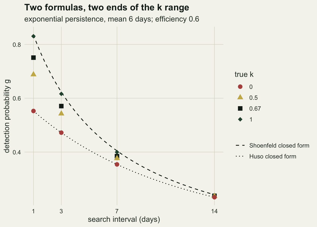
The bracket is widest where searching is most frequent
With trial estimates set to their true values, an estimator’s expected answer divided by the true total is the true g divided by the g the estimator assumes. For a true k between the two conventions, Shoenfeld’s answer is too low and Huso’s too high. The persistence curve used by the estimators is exponential with the right mean; the second and third panels keep that analyst’s model and change the real persistence shape.
br_tab <- expand.grid(interval = intervals, k = k_levels,
                      shape = names(surv_list), stringsAsFactors = FALSE)
br_tab$g <- mapply(function(i, k, s) g_exact(i, k, surv_list[[s]]),
                   br_tab$interval, br_tab$k, br_tab$shape)
br_tab$shoen <- br_tab$g / g_shoenfeld(br_tab$interval, mean_pers, p_eff)
br_tab$huso  <- br_tab$g / g_huso(br_tab$interval, mean_pers, p_eff)
br_of <- function(shape, k, i, col) {
  br_tab[br_tab$shape == shape & br_tab$k == k & br_tab$interval == i, col]
}
exp_name <- "exponential"; w07 <- "Weibull, shape 0.7"; w15 <- "Weibull, shape 1.5"

w07_k0 <- br_tab[br_tab$shape == w07 & br_tab$k == 0, ]
w15_k1 <- br_tab[br_tab$shape == w15 & br_tab$k == 1, ]

ratio_closed <- exp(1 / mean_pers) / (exp(1 / mean_pers) - 1 + p_eff)
ratio_formulas <- g_shoenfeld(1, mean_pers, p_eff) / g_huso(1, mean_pers, p_eff)

bracket_df <- br_tab[br_tab$k == 0.5, ]
bracket_df$shape <- factor(bracket_df$shape, levels = names(surv_list))
bracket_long <- rbind(
  data.frame(bracket_df[, c("interval", "shape")], ratio = bracket_df$shoen,
             estimator = "Shoenfeld (k = 1)"),
  data.frame(bracket_df[, c("interval", "shape")], ratio = bracket_df$huso,
             estimator = "Huso (k = 0)"))
For true k = 0.5 under exponential persistence, Shoenfeld’s expected answer is 0.823 of the true total at daily searches and Huso’s is 1.245. At 3 days the pair is 0.870 and 1.149, at 7 days 0.931 and 1.064, and at 14 days 0.977 and 1.017. Under the wrong convention at the extremes of k the error is larger: Huso’s estimator with a true k of 1 returns 1.503 times the truth at daily searches, and Shoenfeld’s with a true k of 0 returns 0.661.
The ratio of the two closed forms simplifies to e(I/t)/(e(I/t) - 1 + p), which is 1.5119 at daily searches against 1.5119 from the two functions. The reason is the count of chances. A carcass with a mean persistence of 6 days meets several searches when they are a day apart and seldom more than one when they are two weeks apart. With one chance, what happens after a miss cannot matter, and both formulas reduce to the same product of efficiency and persistence. The design that finds the most carcasses is the one whose answer depends most on k.
The bracket is a statement about k given the right persistence model. With a falling scavenging hazard (Weibull shape 0.7, removal concentrated in the first nights) and a true k of 0, which is exactly Huso’s assumption, Huso’s estimator still returns between 0.833 and 0.894 of the truth across the four intervals. With a rising hazard (shape 1.5) and a true k of 1, Shoenfeld’s returns between 1.049 and 1.123. An exponential of the right mean, when the real persistence is not exponential, moves both ends of the bracket in the same direction, and the truth can then sit outside it.
ggplot(bracket_long, aes(interval, ratio, colour = estimator)) +
  geom_hline(yintercept = 1, linetype = "dashed", colour = te_body,
             linewidth = 0.5) +
  geom_line(linewidth = 0.9) +
  geom_point(size = 2.4) +
  facet_wrap(~ shape) +
  scale_colour_manual(values = c("Shoenfeld (k = 1)" = te_forest,
                                 "Huso (k = 0)" = te_rust), name = NULL) +
  scale_x_continuous(breaks = intervals) +
  labs(x = "search interval (days)", y = "estimate / true total",
       title = "The k bracket narrows as searches spread out",
       subtitle = "true k 0.5; dashed: unbiased") +
  theme_datasheet() +
  theme(legend.position = "bottom")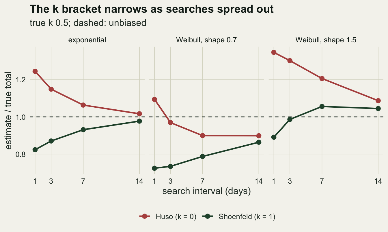
Whole studies with trial carcasses
A real study does not know t or p. Each simulated study below has 100 true deaths in the searched plots, forty persistence trial carcasses followed for up to 28 days (the mean persistence estimated by the censored exponential maximum likelihood, total exposure over removals), and forty efficiency trial carcasses. The efficiency trial carcasses are searched twice: the first search gives p, and the second search of those missed gives an estimate of k that only the last of the estimators below uses. The count found is binomial with the exact g for the true k.
The interval is a parametric bootstrap. Each of 400 replicates redraws the persistence trial from the fitted exponential and the efficiency trial from the fitted p and k, recomputes g, and then draws the total as the count plus a negative binomial number of missed deaths given that g. A fourth version holds g at its estimate and keeps only the count noise, to show what the trial uncertainty contributes. Each cell has 1000 simulated studies.
n_study      <- 1000
n_boot       <- 400
n_pers_trial <- 40
n_eff_trial  <- 40
cens_day     <- 28
m_true       <- 100

fit_tbar <- function(x) colSums(pmin(x, cens_day)) / pmax(1, colSums(x < cens_day))
fit_k <- function(n1, n2, n_trial) {
  p_hat <- n1 / n_trial
  q_hat <- ifelse(n1 < n_trial, n2 / pmax(1, n_trial - n1), p_hat)
  pmin(1, ifelse(n1 > 0, q_hat / pmax(p_hat, 1e-9), 1))
}
col_quant <- function(mat, prob) {
  sorted <- matrix(mat[order(col(mat), mat)], nrow(mat))
  sorted[ceiling(prob * nrow(mat)), ]
}

run_studies <- function(k_true) {
  pers_obs <- matrix(rexp(n_pers_trial * n_study, 1 / mean_pers), n_pers_trial)
  t_hat <- fit_tbar(pers_obs)
  n1 <- rbinom(n_study, n_eff_trial, p_eff)
  n2 <- rbinom(n_study, n_eff_trial - n1, k_true * p_eff)
  p_hat <- n1 / n_eff_trial
  k_hat <- fit_k(n1, n2, n_eff_trial)

  t_boot <- matrix(0, n_boot, n_study)
  for (b in seq_len(n_boot)) {
    redraw <- matrix(rexp(n_pers_trial * n_study,
                          1 / rep(t_hat, each = n_pers_trial)), n_pers_trial)
    t_boot[b, ] <- fit_tbar(redraw)
  }
  n1_boot <- matrix(rbinom(n_boot * n_study, n_eff_trial,
                           rep(p_hat, each = n_boot)), n_boot)
  n2_boot <- matrix(rbinom(n_boot * n_study, n_eff_trial - n1_boot,
                           rep(k_hat * p_hat, each = n_boot)), n_boot)
  p_boot <- n1_boot / n_eff_trial
  k_boot <- fit_k(n1_boot, n2_boot, n_eff_trial)

  one_interval <- function(interval) {
    count <- rbinom(n_study, m_true,
                    g_exact(interval, k_true, surv_list[["exponential"]]))
    summarise_est <- function(g_hat, g_boot, label) {
      m_boot <- matrix(rep(count, each = n_boot), n_boot) +
        matrix(rnbinom(n_boot * n_study, size = rep(count + 1, each = n_boot),
                       prob = g_boot), n_boot)
      lower_q <- col_quant(m_boot, 0.025)
      upper_q <- col_quant(m_boot, 0.975)
      data.frame(k_true = k_true, interval = interval, estimator = label,
                 ratio = mean(count / g_hat) / m_true,
                 coverage = mean(lower_q <= m_true & upper_q >= m_true),
                 width = median(upper_q - lower_q))
    }
    g_h <- g_huso(interval, t_hat, p_hat)
    rbind(
      summarise_est(g_shoenfeld(interval, t_hat, p_hat),
                    g_shoenfeld(interval, t_boot, p_boot), "Shoenfeld (k = 1)"),
      summarise_est(g_h, g_huso(interval, t_boot, p_boot), "Huso (k = 0)"),
      summarise_est(g_h, matrix(rep(g_h, each = n_boot), n_boot),
                    "Huso, count noise only"),
      summarise_est(g_k_series(interval, t_hat, p_hat, k_hat),
                    g_k_series(interval, t_boot, p_boot, k_boot), "k estimated"))
  }
  do.call(rbind, lapply(intervals, one_interval))
}

set.seed(2011)
cov_tab <- do.call(rbind, lapply(c(1, 0.5, 0), run_studies))
cov_of <- function(k, i, est, col) {
  cov_tab[cov_tab$k_true == k & cov_tab$interval == i &
            cov_tab$estimator == est, col]
}
mc_se <- sqrt(0.95 * 0.05 / n_study)
k_est_cov <- cov_tab$coverage[cov_tab$estimator == "k estimated"]
huso_noise <- cov_tab$coverage[cov_tab$estimator == "Huso, count noise only" &
                                 cov_tab$k_true == 0]
huso_full  <- cov_tab$coverage[cov_tab$estimator == "Huso (k = 0)" &
                                 cov_tab$k_true == 0]
The Monte Carlo standard error of a coverage near 0.95 is 0.0069 with 1000 studies.
Start where Huso’s assumption is true. With k = 0 the Huso interval covers the true total in 0.934 to 0.954 of studies across the four intervals. The same point estimate with an interval that ignores the trial uncertainty covers in only 0.739 to 0.827. Forty trial carcasses of each kind leave enough uncertainty in g that the count noise alone is the smaller part of the interval: at 7-day searches the median width is 86 deaths with the trials propagated and 53 without.
Now the middle case, a true k of 0.5. At daily searches the Shoenfeld interval covers in 0.345 of studies and is the narrowest of the four, with a median width of 22 deaths: a confident answer centred at 0.830 of the truth. The Huso interval covers in 0.652, with its mean estimate at 1.270 of the truth; its interval is wider because a small g is uncertain in relative terms, and the width partly hides the bias. At 14-day searches both conventions cover in 0.946 and 0.948.
The estimator that uses the second search of the trial carcasses covers in 0.933 to 0.958 of studies over all twelve cells, including the two ends of k where one of the conventions is correct. The price appears at k = 1: at daily searches its median width is 33 deaths against 24 for Shoenfeld, and its mean estimate is 1.021 of the truth. At k = 0 there is no price, because the estimated k is zero in every trial (next section) and the interval matches Huso’s: at 7-day searches its median width is 85 deaths against 86.
cov_plot <- cov_tab
cov_plot$panel <- factor(paste("true k =", cov_plot$k_true),
                         levels = paste("true k =", c(1, 0.5, 0)))
ggplot(cov_plot, aes(factor(interval), coverage, colour = estimator)) +
  annotate("rect", xmin = -Inf, xmax = Inf, ymin = 0.95 - 2 * mc_se,
           ymax = 0.95 + 2 * mc_se, fill = te_line, alpha = 0.7) +
  geom_hline(yintercept = 0.95, linetype = "dashed", colour = te_body,
             linewidth = 0.4) +
  geom_point(aes(shape = estimator), size = 2.6, position = position_dodge(width = 0.6)) +
  facet_wrap(~ panel) +
  scale_colour_manual(values = c("Shoenfeld (k = 1)" = te_forest,
                                 "Huso (k = 0)" = te_rust,
                                 "Huso, count noise only" = te_gold,
                                 "k estimated" = te_ink), name = NULL) +
  scale_shape_manual(values = c("Shoenfeld (k = 1)" = 16, "Huso (k = 0)" = 16,
                                "Huso, count noise only" = 16, "k estimated" = 17),
                     name = NULL) +
  scale_y_continuous(limits = c(0, 1)) +
  labs(x = "search interval (days)", y = "interval coverage",
       title = "The estimated k stays near 0.95 in every cell",
       subtitle = "40 persistence and 40 efficiency trial carcasses per study") +
  theme_datasheet() +
  theme(legend.position = "bottom") +
  guides(colour = guide_legend(nrow = 2), shape = guide_legend(nrow = 2))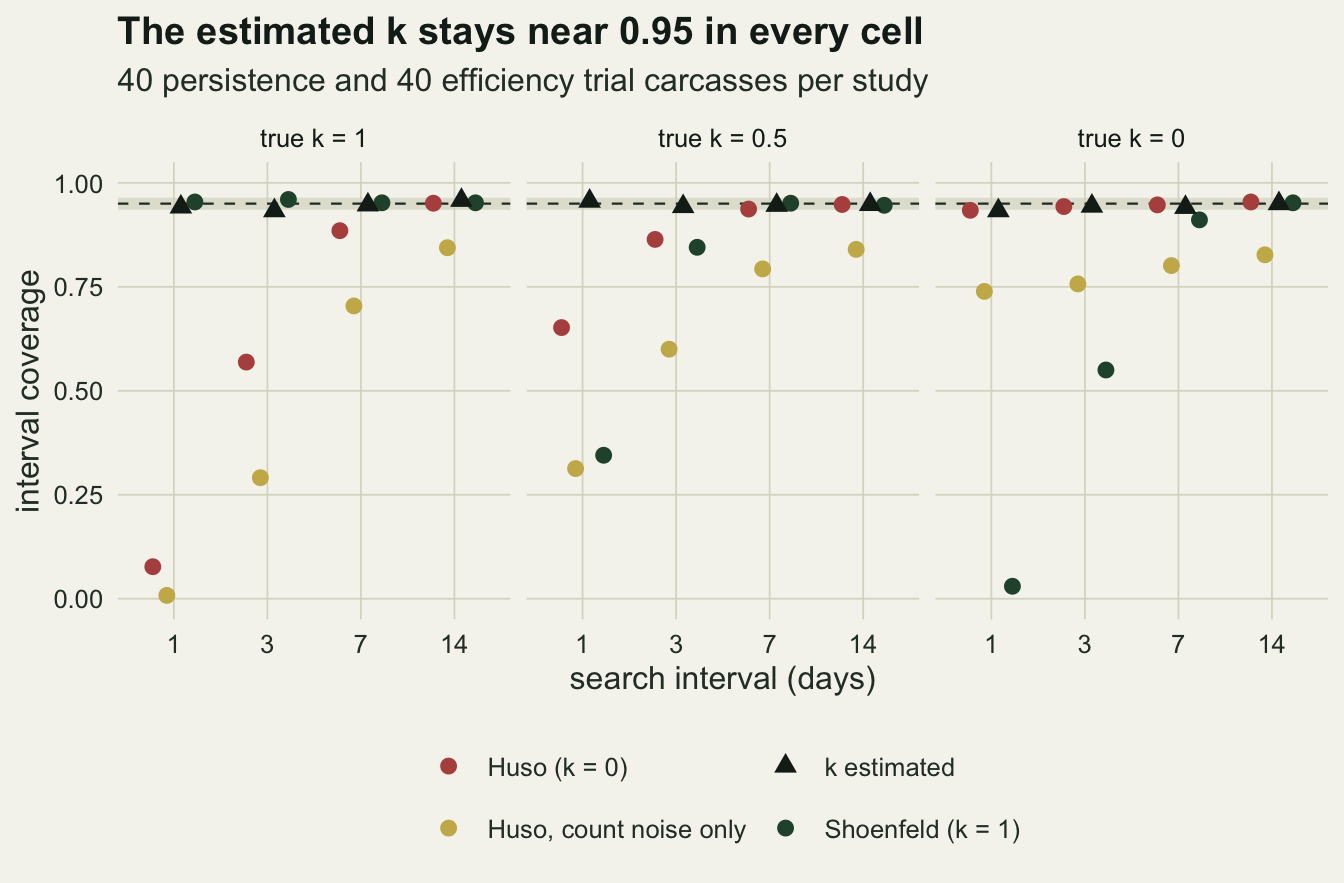
A second search of the trial carcasses identifies k
A single-search efficiency trial yields one binomial proportion, and every value of k fits it equally well, because k acts only on carcasses that have already been missed. The Korner-Nievergelt formula carries k as a parameter; the GenEst models of Dalthorp and colleagues estimate it when trial carcasses missed on one search are left in place for later searches. The simplest version is the one used above: search each trial carcass twice. The first search estimates p, and the share of the missed carcasses found on the second estimates kp, so k is their ratio, capped at one. This assumes the trial carcasses are still present at the second search, which a trial can arrange by checking them.
set.seed(4)
n_draw <- 5000
k_grid <- expand.grid(k_true = c(0, 0.5, 1), n_trial = c(40, 100))
k_draws <- do.call(rbind, lapply(seq_len(nrow(k_grid)), function(i) {
  n1 <- rbinom(n_draw, k_grid$n_trial[i], p_eff)
  n2 <- rbinom(n_draw, k_grid$n_trial[i] - n1, k_grid$k_true[i] * p_eff)
  data.frame(k_true = k_grid$k_true[i], n_trial = k_grid$n_trial[i],
             k_hat = fit_k(n1, n2, k_grid$n_trial[i]))
}))
k0_zero <- sum(k_draws$k_hat[k_draws$k_true == 0] == 0)
k0_all <- sum(k_draws$k_true == 0)
k_sum <- function(k, n, fun) fun(k_draws$k_hat[k_draws$k_true == k & k_draws$n_trial == n])
q05 <- function(v) quantile(v, 0.05, names = FALSE)
q95 <- function(v) quantile(v, 0.95, names = FALSE)
at_one <- function(v) mean(v == 1)
missed_40 <- n_eff_trial * (1 - p_eff)
With forty trial carcasses and a true k of 0.5, the 90 per cent range of the estimate is 0.20 to 0.85, because on average only 16 carcasses are missed on the first search and the second search works on those. With a hundred carcasses the range narrows to 0.30 to 0.72. With a true k of 1 the estimate hits the cap in 0.547 of forty-carcass trials and averages 0.910, a downward pull that explains the small upward shift of the k-estimated total in that case. With a true k of 0 no missed carcass is ever found again and the estimate is zero in 10000 of 10000 simulated trials.
That the imprecise forty-carcass k still gave coverage within 0.017 of 0.95 in the previous section is the practical result. The interval does not need k to be known well; it needs the uncertainty in k to be carried into g, and at long intervals g barely depends on k at all.
khat_plot <- k_draws[k_draws$k_true > 0, ]
khat_plot$row_lab <- factor(paste(khat_plot$n_trial, "trial carcasses"),
                            levels = c("40 trial carcasses", "100 trial carcasses"))
khat_plot$col_lab <- paste("true k =", khat_plot$k_true)
true_lines <- unique(khat_plot[, c("row_lab", "col_lab", "k_true")])
ggplot(khat_plot, aes(k_hat)) +
  geom_histogram(binwidth = 0.05, boundary = 0, fill = te_forest,
                 colour = te_paper, linewidth = 0.2) +
  geom_vline(data = true_lines, aes(xintercept = k_true), colour = te_rust,
             linetype = "dashed", linewidth = 0.7) +
  facet_grid(row_lab ~ col_lab) +
  labs(x = "estimated k", y = "simulated trials",
       title = "What a second search buys",
       subtitle = "efficiency 0.6; k capped at one") +
  theme_datasheet()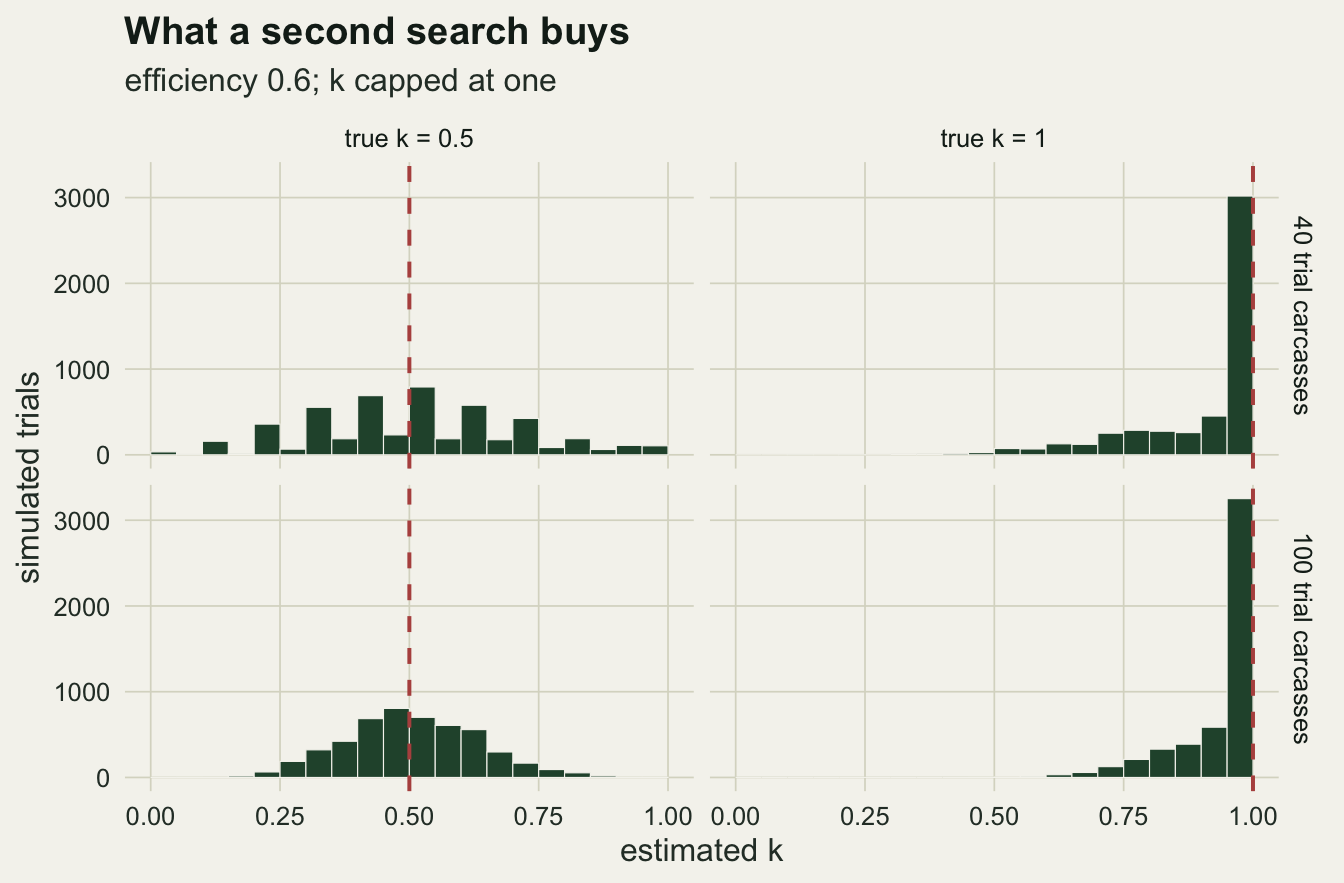
What to report
State which k the estimator assumes, in those words. A total computed with the Huso formula is a total under the assumption that a missed carcass is never found, and one computed with the Shoenfeld formula assumes it is found as easily as a fresh one. Readers of a monitoring report cannot recover that from the phrase “corrected for searcher efficiency and carcass persistence”.
Report the search interval next to the mean persistence. Their ratio tells a reader how many chances a typical carcass had. Under the design here, at daily searches the two conventions gave 0.823 and 1.245 of the truth for a middle k, and at 14 days 0.977 and 1.017. A frequent-search study that reports one number without k has chosen a point in a wide range.
Leave missed efficiency trial carcasses in place for at least one more search, and report the estimated k with the trial size. That costs a second visit to carcasses already laid out, and in these simulations it was the difference between coverage of at least 0.933 and the Shoenfeld coverage of 0.345 at daily searches with a true k of 0.5.
Propagate the trial uncertainty into the interval. Even with the correct k, an interval built from the count alone covered in at most 0.827 of studies with forty trial carcasses of each kind.
Report the persistence model and how it was chosen. A decreasing scavenging hazard modelled as an exponential of the right mean moved both conventions downward in the bracket calculation, so a correct k does not rescue a wrong persistence curve.
Honest limits
Efficiency here changes by the same factor after every miss and is the same for every carcass. Real carcasses differ in size and in the vegetation they fall into, and a population of easy and hard carcasses produces a falling efficiency across searches without any single carcass changing. The factor k absorbs that heterogeneity only approximately; with strong heterogeneity the two-search trial estimates an average decline that need not hold at the fifth or tenth search, which is where daily searching puts most of its weight.
The two-search trial assumes its carcasses persist until the second search. If some are scavenged in between, a carcass not found at the second search may simply be gone, and k is underestimated unless persistence is checked independently. Placing trial carcasses and checking them separately from the blind search, or modelling removal and detection jointly, handles that; neither is simulated here.
Persistence trials record removal times exactly, up to a 28-day censoring point. Field trials check carcasses on set days, so removal is interval censored, and the exponential mean fitted to such data is a little less precise than here. The effect on coverage was not measured.
The estimator with k estimated uses an unbounded season, so it inherits the end-of-season gap measured for the Shoenfeld form (up to 1.2 per cent); the exact g for an 84-day season would remove it. The simulated deaths arrive uniformly. Fatalities at wind turbines cluster in migration pulses and on low-wind nights, and a pulse just before the last search behaves like the end of the season.
The searched area is treated as the whole kill zone. Real plots miss carcasses that fall outside them, and the correction for unsearched area is a separate factor with its own uncertainty that multiplies everything above. The bootstrap here also treats the persistence and efficiency trials as drawn from the same carcass population as the fatalities, while trials often use surrogate species of a different size.
Coverage was measured for one true total, one efficiency and one persistence mean. The ratio of the two closed forms reduces to e(I/t)/(e(I/t) - 1 + p), which grows as efficiency falls or persistence lengthens, so the bracket widens with either change; the numbers above belong to this design only.
References
Huso MMP 2011 Environmetrics 22(3):318-329 (10.1002/env.1052)
Korner-Nievergelt F, Korner-Nievergelt P, Behr O, Niermann I, Brinkmann R, Hellriegel B 2011 Wildlife Biology 17(4):350-363 (10.2981/10-121)
Dalthorp D, Madsen L, Huso MM, Rabie P, Wolpert R, Studyvin J, Simonis J, Mintz J 2018 US Geological Survey Techniques and Methods 7-A2 (10.3133/tm7a2)
Horvitz DG, Thompson DJ 1952 Journal of the American Statistical Association 47(260):663-685 (10.1080/01621459.1952.10483446)