Horvitz-Thompson for adaptive samples

Estimate abundance from an adaptive cluster sample with the Horvitz-Thompson estimator: network inclusion probabilities in R, and why it beats Hansen-Hurwitz.

The previous post built adaptive cluster sampling and fixed the biased naive mean with the Hansen-Hurwitz estimator. Hansen-Hurwitz is unbiased and easy to compute, but it is not the tightest estimator the design allows. This post derives the alternative: the Horvitz-Thompson estimator, which works from the probability that each network makes it into the sample. It is a little more work to set up and it wins on precision.

The idea is the same one that runs through all unequal-probability sampling (Horvitz and Thompson 1952): if you can write down the probability that each thing you observed had of being observed, you can weight each observation by the inverse of that probability and recover an unbiased total. In adaptive cluster sampling the “things” are networks, and their inclusion probabilities have a clean closed form.

The probability a network gets into the sample

A network of m units is included in the sample if and only if the initial simple random sample lands on at least one of its units. The complement is easier to count: the probability the initial sample of 30 units avoids the whole network. So the inclusion probability of a network of size \(m\) is

\[ \alpha = 1 - \frac{\binom{N-m}{n_1}}{\binom{N}{n_1}}, \]

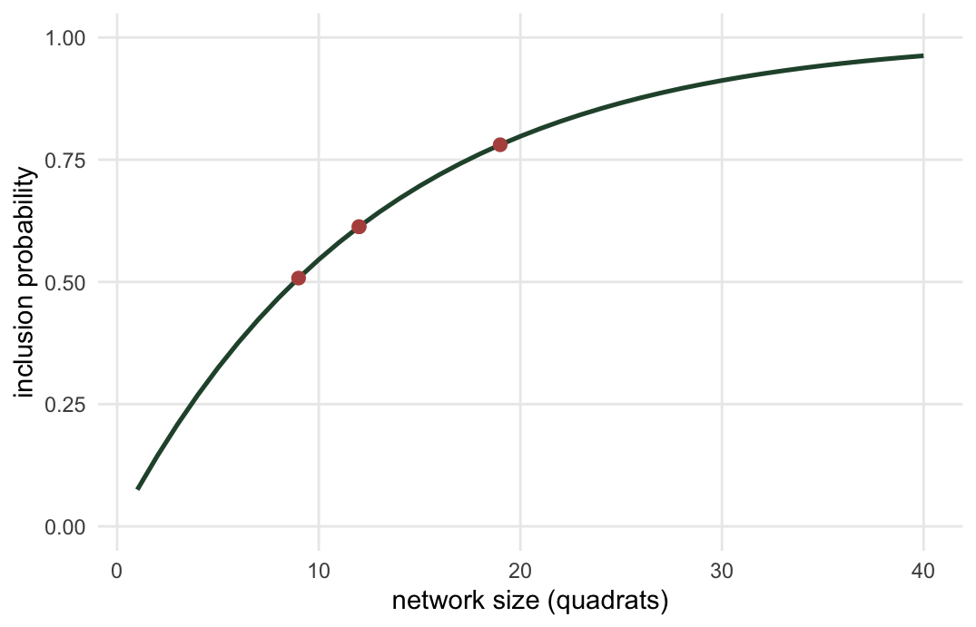
with \(N\) the number of quadrats and \(n_1\) the initial sample size. Bigger networks are far more likely to be hit; a single quadrat is included only with the plain initial probability \(n_1/N\).

alpha <- function(m, N, n1) 1 - choose2(N - m, n1) / choose2(N, n1)
m_big <- max(nets$m)                        # the largest occupied network
c(largest_network = m_big,
  alpha_largest = round(alpha(m_big, N, n1), 4),
  alpha_single  = round(alpha(1, N, n1), 4),   # = n1 / N
  n1_over_N     = round(n1 / N, 4))

largest_network   alpha_largest    alpha_single       n1_over_N 
        19.0000          0.7806          0.0750          0.0750 

The largest occupied network here spans 19 quadrats and has inclusion probability 0.7806: with 30 initial draws it is caught almost four times out of five. A lone quadrat has probability only 0.0750, exactly \(n_1/N\). That spread in inclusion probabilities is what the estimator has to correct for.

Attaching package: 'ggplot2'

The following object is masked _by_ '.GlobalEnv':

    alpha

Figure 1: Inclusion probability against network size for the initial sample of 30 quadrats. A single quadrat enters with probability n1/N; large clusters are nearly certain to be caught.

The Horvitz-Thompson estimator

With inclusion probabilities in hand, the estimator writes itself. Take the distinct networks the initial sample intersected, divide each network’s total by its inclusion probability, add them up, and divide by the number of quadrats for the mean.

horvitz_thompson <- function(nets, hit, N, n1) {
  a <- alpha(nets$m[hit], N, n1)
  sum(nets$tot[hit] / a) / N
}
set.seed(7); d1 <- acs_draw(pop, nets, ubn, n1)
horvitz_thompson(nets, d1$hit, N, n1)

[1] 0.244039

The word distinct is doing real work. If two of your initial units land in the same cluster, that network was still included once, so it enters the sum once, weighted by its single inclusion probability. This is where Horvitz-Thompson parts company with Hansen-Hurwitz, which effectively counts a network once per initial hit.

Why it beats Hansen-Hurwitz

On a clustered population the initial sample often hits the same network more than once: there are only a few networks and 30 initial draws.

set.seed(202); B <- 20000L; multi <- logical(B)
for (b in 1:B) {
  init <- sample.int(N, n1); tab <- table(nets$net_id[init])
  multi[b] <- any(tab > 1 & nets$net_is_sat[as.integer(names(tab))])
}
mean(multi)          # fraction of draws with a multiply-hit occupied network

[1] 0.71445

An occupied network is hit more than once in 71% of draws. Hansen-Hurwitz counts each of those hits, so the same cluster enters the average two or three times, and that repetition adds variance for no information. Horvitz-Thompson counts the cluster once. In estimation-theory terms the Horvitz-Thompson estimator is a function of the distinct networks and their values, which is the minimal sufficient statistic for this design, while Hansen-Hurwitz is not; the Rao-Blackwell versions of both improve on the originals (Salehi 1999).

mc <- function(pop, nets, ubn, n1, B, seed) {
  set.seed(seed); hh <- ht <- numeric(B); cov_ht <- logical(B); neg <- 0L
  mu <- mean(pop$y)
  for (b in 1:B) {
    d <- acs_draw(pop, nets, ubn, n1)
    hh[b] <- d$hh; ht[b] <- d$ht
    vt <- ht_var(pop, nets, d$hit, n1)
    if (!is.na(vt) && vt < 0) neg <- neg + 1L
    cov_ht[b] <- if (is.na(vt) || vt <= 0) NA else abs(d$ht - mu) <= 1.96 * sqrt(vt)
  }
  list(hh = hh, ht = ht, cov_ht = cov_ht, neg = neg)
}
M <- mc(pop, nets, ubn, n1 = 30L, B = 20000L, seed = 202L)
c(bias_ht = round(mean(M$ht) - mu, 5),
  sd_hh = round(sd(M$hh), 4), sd_ht = round(sd(M$ht), 4),
  var_ratio_ht_over_hh = round(var(M$ht) / var(M$hh), 3))

             bias_ht                sd_hh                sd_ht 
            -0.00003              0.13490              0.10370 
var_ratio_ht_over_hh 
             0.59100 

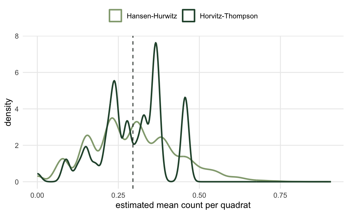
Both estimators are unbiased: the Horvitz-Thompson bias over 20,000 samples is -0.00003. But the Horvitz-Thompson variance is 0.591 times the Hansen-Hurwitz variance, a standard error of 0.1037 against 0.1349, or about 23% narrower. On this population the improvement is worth having, and Salehi (2003) recommends Horvitz-Thompson as the default despite the heavier bookkeeping.

Figure 2: Sampling distributions of the two unbiased estimators over 20,000 initial samples. Both centre on the truth; the Horvitz-Thompson estimator is the tighter of the two.

The interval is still the weak point

More precise does not mean better calibrated. The unbiased Horvitz-Thompson variance estimator uses pairwise network inclusion probabilities, and on a skewed population the normal interval built from it undercovers, a touch worse than the Hansen-Hurwitz one from the previous post.

c(ht_interval_cover = round(ht_cover, 3),
  negative_variance_estimates = M$neg)

          ht_interval_cover negative_variance_estimates 
                      0.883                       0.000 

The interval reaches only about 88.3% cover here. No variance estimate came out negative on this population, but the Horvitz-Thompson variance estimator can go negative in general, which is one more reason field guidance leans on a bootstrap interval for adaptive samples. The point estimate is excellent; the interval needs care. The next post steps back from the estimator to the design itself and asks the question that decides whether any of this is worth doing: when does adaptive sampling actually beat a simple random sample?

Related tutorials

• Adaptive cluster sampling in R
• When does adaptive sampling pay?
• Checking an adaptive sampling design
• Unequal-probability spatial sampling

References

Horvitz DG, Thompson DJ 1952 J Am Stat Assoc 47(260):663-685 (10.1080/01621459.1952.10483446)

Thompson SK 1990 J Am Stat Assoc 85(412):1050-1059 (10.1080/01621459.1990.10474975)

Salehi MM 1999 Environ Ecol Stat 6(2):183-195 (10.1023/A:1009670205509)

Salehi MM 2003 Environ Ecol Stat 10(1):115-127 (10.1023/A:1021989509323)

Thompson SK, Seber GAF 1996 Adaptive Sampling. Wiley (ISBN 978-0-471-55871-2)