When does adaptive sampling pay?

Adaptive cluster sampling beats simple random sampling on some populations and loses on others. Compare them fairly in R and find the condition that decides it.

The first two posts in this thread built adaptive cluster sampling and two unbiased estimators for it. Both showed the design in a flattering light, because both compared estimators on the same design. This post asks the harder question: should you run the design at all, or would a simple random sample of the same effort do better?

The answer turns on how you count effort, and the two reasonable ways of counting give opposite verdicts on the same population. That is not a trick; it is the central practical fact about adaptive designs, and getting it wrong is how a survey ends up over budget and less precise than the plain design it replaced.

Two ways to count the cost

An adaptive design starts from an initial sample of 30 quadrats and then grows. So there are two honest baselines. You can give simple random sampling the same initial sample size, which asks “given that I am going out to 30 randomly chosen quadrats, is it worth expanding around the ones with animals?” Or you can give it the same total number of quadrats actually visited, which asks “given a fixed field budget of quadrat-visits, which design spends it better?”

srs_mean <- function(pop, n, B, seed) {
  set.seed(seed); N <- pop$N; y <- pop$y
  vapply(1:B, function(b) mean(y[sample.int(N, n)]), numeric(1))
}
acs_mc <- function(pop, nets, n1, B, seed) {
  set.seed(seed); ht <- nf <- numeric(B)
  for (b in 1:B) { d <- acs_draw(pop, nets, n1); ht[b] <- d$ht; nf[b] <- d$n_final }
  list(ht = ht, nf = nf)
}
A    <- acs_mc(pop, nets, n1, 20000L, 202L)
srs1 <- srs_mean(pop, n1, 20000L, 303L)        # same INITIAL sample size
c(sd_srs_30 = round(sd(srs1), 4), sd_adaptive = round(sd(A$ht), 4),
  efficiency = round(var(srs1) / var(A$ht), 2))

  sd_srs_30 sd_adaptive  efficiency 
     0.1699      0.1037      2.6800 

At equal initial effort the adaptive design is 2.7 times as efficient: a standard error of 0.1037 against 0.1699. If you stopped here you would conclude that adaptive sampling is a large free gain.

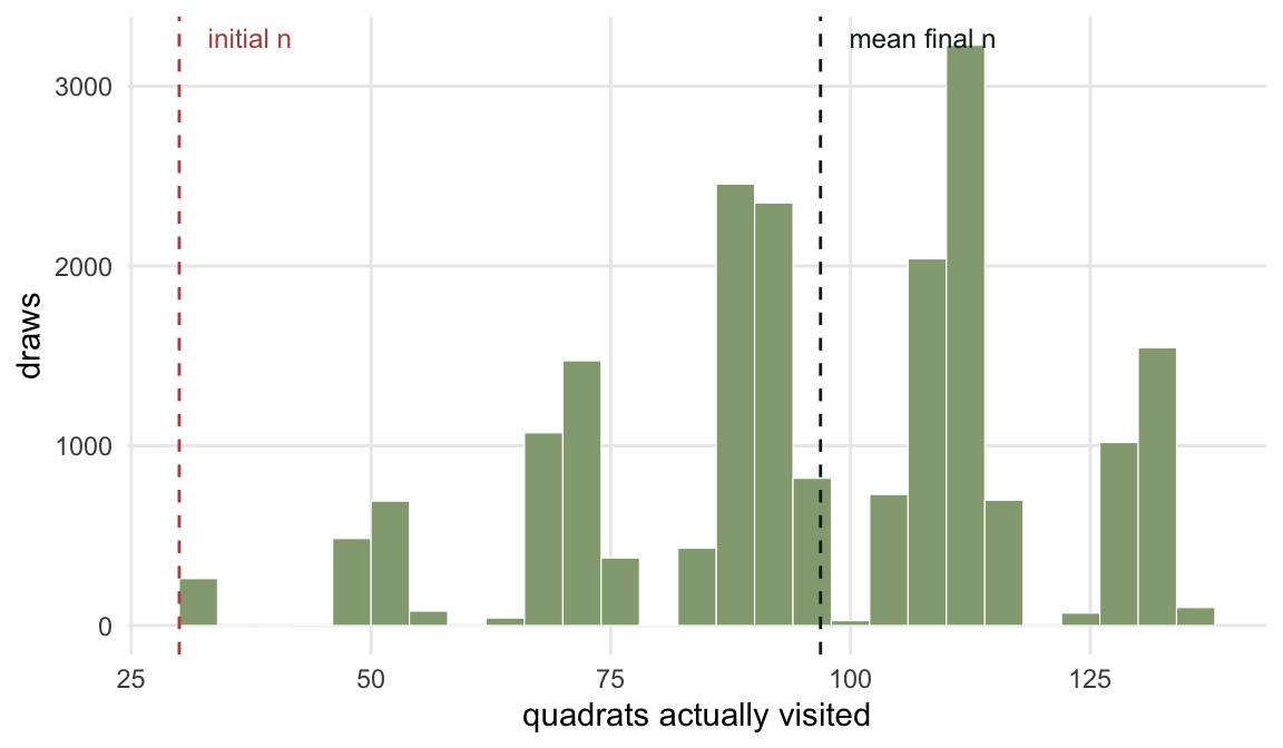
It is not free. The expansion visits extra quadrats, and those visits are the real currency of field work.

c(mean_final_n = round(mean(A$nf), 1), sd_final_n = round(sd(A$nf), 1),
  min_final_n = min(A$nf), max_final_n = max(A$nf))

mean_final_n   sd_final_n  min_final_n  max_final_n 
        96.9         23.0         30.0        137.0 

Figure 1: Distribution of the realised sample size over 20,000 adaptive draws. The initial sample is fixed at 30 quadrats; what you actually visit is not, and it ranges from 30 to over 130.

On average the design visits 97 quadrats, more than three times the initial 30, and in the worst draw it visited 137. So the fair budget comparison is against a simple random sample of about 97 quadrats.

ne   <- round(mean(A$nf))
srsE <- srs_mean(pop, ne, 20000L, 404L)        # same TOTAL effort
c(n = ne, sd_srs = round(sd(srsE), 4), sd_adaptive = round(sd(A$ht), 4),
  efficiency = round(var(srsE) / var(A$ht), 2))

          n      sd_srs sd_adaptive  efficiency 
    97.0000      0.0861      0.1037      0.6900 

The verdict flips. At equal total effort the efficiency is 0.69, which is below one: on this population a plain simple random sample of 97 quadrats beats the adaptive design that visits 97 quadrats on average. The adaptive gain at equal initial effort was real, but it was bought with visits, and buying the same visits outright buys more precision.

So when does it pay?

The design earns its keep when the species is both rare and strongly clumped, because then the expansion is triggered rarely and, when it fires, it lands you inside the few units that carry the information. Push the clumping down and the design starts expanding everywhere for little return.

To test that, hold total abundance fixed and vary only how tightly the individuals are packed. The variance-to-mean ratio of the counts measures the clumping: it is one for a random (Poisson) field and rises with aggregation.

sweep_agg <- function(spreads, B = 8000L, seed = 11L) {
  do.call(rbind, lapply(spreads, function(s) {
    p <- make_population(spread = s, seed = 55L); nn <- build_networks(p, 1L)
    r <- acs_mc(p, nn, n1, B, seed)
    ne <- round(mean(r$nf)); sr <- srs_mean(p, ne, B, seed + 1L)
    data.frame(spread = s, total = sum(p$y), vmr = vmr(p),
               occupancy = mean(p$y >= 1), mean_final_n = mean(r$nf),
               efficiency = var(sr) / var(r$ht))
  }))
}
sw <- sweep_agg(c(0.5, 0.9, 1.5, 2.5))
round(sw, 3)

  spread total   vmr occupancy mean_final_n efficiency
1    0.5   133 8.704     0.062       51.005      1.181
2    0.9   133 3.729     0.128       94.874      0.745
3    1.5   133 1.875     0.205      139.511      0.874
4    2.5   133 1.453     0.232      136.931      0.341

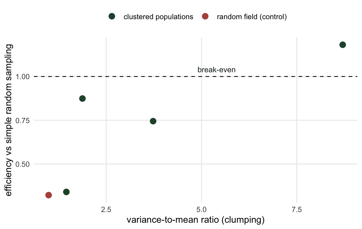
All four populations hold the same 133 individuals; only their packing differs. The tightest one (variance-to-mean ratio 8.7, occupancy 6.2%) is the only case where the efficiency clears one, at 1.18. Notice why: with the animals in a few tiny knots the design almost never triggers, so it visits only 51 quadrats. It stays cheap and it finds the knots. As the packing loosens, the efficiency falls to 0.34 at a ratio of 1.5.

Figure 2: Efficiency against clumping, at equal total effort. Only the most strongly aggregated population puts adaptive sampling above the break-even line; the relationship is not a clean ramp, because the design’s cost moves with the clumping too.

An honest limit: it is not a clean ramp

The four points do not lie on a tidy increasing curve. Efficiency is 0.74 at a ratio of 3.7 but 0.87 at a ratio of 1.9, which reverses the expected order. That is not simulation noise; it repeats across seeds.

The reason is that clumping moves two things at once. It changes how much information sits in the networks, and it changes how much the design expands: the mean final sample size runs 51, 95, 140, 137 across the four populations. Since the comparison re-baselines simple random sampling to whatever the adaptive design happened to cost, the yardstick moves with the design. There is no single number that summarises “aggregation” and predicts efficiency on its own, which is why the practical advice is to simulate your own case rather than trust a rule of thumb.

The control confirms the easy half of the story. On a random field of the same mean, with a variance-to-mean ratio of 0.99, the adaptive design still expands to 87 quadrats (occupancy is 26%, so it triggers constantly) and returns an efficiency of 0.32. When there are no clusters to find, expanding is a pure cost.

What to take to the field

Run the design when the species is rare enough that expansion stays rare, and clumped enough that hitting one occupied quadrat tells you where more are. Sparse, patchy, hard-to-find organisms are exactly the case Thompson and Seber (1996) had in mind, and where field applications have paid off (Smith and colleagues 1995). Outside that regime, a well-spread fixed design is the better buy.

Before committing, simulate your own population, and budget for the sample size you might actually get rather than the one you planned. The next post turns that into three concrete checks you can run before the field season starts.

Related tutorials

• Adaptive cluster sampling in R
• Horvitz-Thompson for adaptive samples
• Checking an adaptive sampling design
• Allocating effort across strata

References

Thompson SK 1990 J Am Stat Assoc 85(412):1050-1059 (10.1080/01621459.1990.10474975)

Thompson SK 1991 Biometrics 47(3):1103-1115 (10.2307/2532662)

Smith DR, Conroy MJ, Brakhage DH 1995 Biometrics 51(2):777-788 (10.2307/2532964)

Brown JA 2003 Environ Ecol Stat 10(1):95-105 (10.1023/A:1021933424344)

Thompson SK, Seber GAF 1996 Adaptive Sampling. Wiley (ISBN 978-0-471-55871-2)