---
title: "Checking an adaptive sampling design"
description: "Three checks before you run adaptive cluster sampling in the field: the condition threshold, the budget you might actually spend, and network double-counting."
date: "2026-06-27 14:00"
date-modified: "2026-09-27"
categories: [R, adaptive sampling, survey design, model checking, ecology tutorial]
image: thumbnail.png
image-alt: "A curve showing the probability that an adaptive sample exceeds a given number of quadrats, falling from near certainty at small budgets to a small tail at large ones."
---
*Corrected 27 September 2026: the threshold figure caption said moving right along the curve buys a cheaper survey; it is moving left. The double-counting caption said the slip adds no noise; the figure shows it also widens the distribution.*
Adaptive cluster sampling has more moving parts than it looks. You choose a condition, you choose an initial sample size, and the design decides for itself how much field work you end up doing. Each of those is a place where a survey can go wrong quietly. This post runs three checks on the design built in [the first post of this thread](../adaptive-cluster-sampling/): one on the condition, one on the budget, and one on the arithmetic of the estimator.
All three are cheap to run before the field season, and all three have caught real problems.
```{r}
#| label: setup
#| code-fold: true
#| code-summary: "Setup: packages, colours and plot theme"
#| results: hide
#| message: false
#| warning: false
options(digits = 6)

make_population <- function(side = 20L, n_clusters = 5L, per_cluster = 22,
                            spread = 0.9, seed = 101L) {
  set.seed(seed); N <- side * side; y <- integer(N)
  cx0 <- runif(n_clusters, 2, side - 1); cy0 <- runif(n_clusters, 2, side - 1)
  for (k in seq_len(n_clusters)) {
    np <- rpois(1, per_cluster); if (np == 0) next
    cx <- pmin(pmax(round(rnorm(np, cx0[k], spread)), 1), side)
    cy <- pmin(pmax(round(rnorm(np, cy0[k], spread)), 1), side)
    cell <- (cy - 1) * side + cx
    tb <- table(cell); idx <- as.integer(names(tb)); y[idx] <- y[idx] + as.integer(tb)
  }
  list(side = side, N = N, y = y)
}
rook <- function(i, side) {
  x <- ((i - 1) %% side) + 1L; yy <- ((i - 1) %/% side) + 1L
  nb <- integer(0)
  if (x > 1) nb <- c(nb, i - 1L); if (x < side) nb <- c(nb, i + 1L)
  if (yy > 1) nb <- c(nb, i - side); if (yy < side) nb <- c(nb, i + side)
  nb
}
build_networks <- function(pop, cval = 1L) {
  side <- pop$side; N <- pop$N; y <- pop$y; sat <- y >= cval
  net_id <- integer(N); cur <- 0L; seen <- logical(N)
  for (i in seq_len(N)) {
    if (seen[i]) next
    if (!sat[i]) { cur <- cur + 1L; net_id[i] <- cur; seen[i] <- TRUE; next }
    cur <- cur + 1L; stack <- i; seen[i] <- TRUE; net_id[i] <- cur
    while (length(stack)) {
      u <- stack[length(stack)]; stack <- stack[-length(stack)]
      for (v in rook(u, side)) if (!seen[v] && sat[v]) {
        seen[v] <- TRUE; net_id[v] <- cur; stack <- c(stack, v) }
    }
  }
  m <- as.integer(table(net_id)); tot <- as.numeric(tapply(y, net_id, sum))
  list(net_id = net_id, m = m, tot = tot, sat = sat,
       net_mean_of_unit = (tot / m)[net_id],
       net_is_sat = as.logical(tapply(sat, net_id, function(z) z[1])))
}
choose2 <- function(a, b) { out <- exp(lchoose(a, b)); out[b < 0 | b > a] <- 0; out }

acs_draw <- function(pop, nets, n1) {
  N <- pop$N; side <- pop$side
  init <- sample.int(N, n1); hit <- unique(nets$net_id[init])
  in_s <- logical(N); in_s[init] <- TRUE
  ubn <- split(seq_len(N), nets$net_id)
  for (k in hit) { uk <- ubn[[k]]; in_s[uk] <- TRUE
    if (nets$net_is_sat[k]) for (u in uk) for (v in rook(u, side)) in_s[v] <- TRUE }
  a <- 1 - choose2(N - nets$m[hit], n1) / choose2(N, n1)
  list(ht = sum(nets$tot[hit] / a) / N, n_final = sum(in_s))
}
srs_mean <- function(pop, n, B, seed) {
  set.seed(seed); N <- pop$N; y <- pop$y
  vapply(1:B, function(b) mean(y[sample.int(N, n)]), numeric(1))
}

pop <- make_population(); nets <- build_networks(pop, 1L)
N <- pop$N; mu <- mean(pop$y); n1 <- 30L
library(ggplot2)
te_canvas <- theme(plot.background  = element_rect(fill = "#f5f4ee", colour = NA),
                   panel.background = element_rect(fill = "#f5f4ee", colour = NA))
```
## Check 1: is the condition set where you think it is?
The condition decides when the crew expands to the neighbours. Presence (a count of at least one) is the obvious choice, but it is a choice, and raising it changes the design more than people expect. Sweep it and watch what moves.
```{r}
#| label: threshold-sweep
#| echo: true
sweep_threshold <- function(cvals, B = 12000L) {
  do.call(rbind, lapply(cvals, function(cv) {
    nn <- build_networks(pop, cval = cv)
    set.seed(21); ht <- nf <- numeric(B)
    for (b in 1:B) { d <- acs_draw(pop, nn, n1); ht[b] <- d$ht; nf[b] <- d$n_final }
    ne <- round(mean(nf)); sr <- srs_mean(pop, ne, B, 22L)
    data.frame(condition = cv, networks = sum(nn$net_is_sat),
               mean_final_n = mean(nf), se = sd(ht),
               efficiency = var(sr) / var(ht))
  }))
}
th <- sweep_threshold(1:3)
round(th, 3)
```
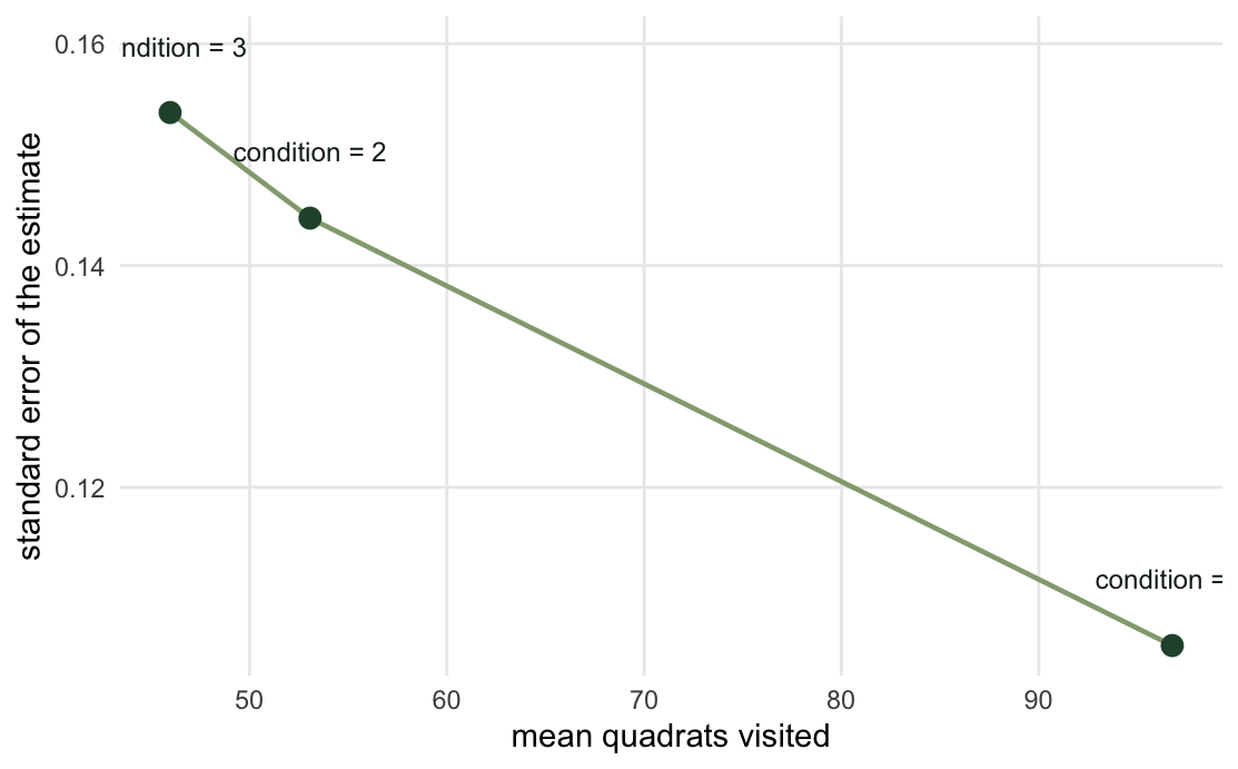
Two things move in opposite directions. Raising the condition from `r th$condition[1]` to `r th$condition[3]` cuts the field cost sharply, from `r sprintf("%.0f", th$mean_final_n[1])` quadrats down to `r sprintf("%.0f", th$mean_final_n[3])`, because the design stops chasing the sparse edges of each patch. Efficiency per unit of effort rises with it, from `r sprintf("%.2f", th$efficiency[1])` to `r sprintf("%.2f", th$efficiency[3])`, although on another draw of the same simulation it can fall instead.
But the standard error goes the wrong way: `r sprintf("%.4f", th$se[1])` at a condition of one, `r sprintf("%.4f", th$se[3])` at three, about `r sprintf("%.0f%%", 100 * (th$se[3] / th$se[1] - 1))` worse. A stricter condition gives you a cheaper survey and a vaguer answer. If you read only the efficiency column you would tighten the condition and quietly lose precision.
```{r}
#| label: fig-threshold
#| echo: false
#| fig-cap: "The condition threshold trades cost against precision. Moving left along the curve buys a cheaper survey and pays for it with a wider standard error."
#| fig-alt: "Three labelled points joined by a line, with mean final sample size on the x axis and standard error on the y axis. As the condition rises from one to three the points move up and to the left: fewer quadrats, a wider standard error."
#| fig-width: 5.8
#| fig-height: 3.6
ggplot(th, aes(mean_final_n, se)) +
geom_line(colour = "#93a87f", linewidth = 0.8) +
geom_point(colour = "#275139", size = 3) +
geom_text(aes(label = paste0("condition = ", condition), hjust = c(1, 0, 0)),
nudge_x = c(-1.2, 1.2, 1.2), nudge_y = 0.006, size = 3.2, colour = "#16241d") +
scale_x_continuous(expand = expansion(mult = 0.14)) +
scale_y_continuous(expand = expansion(mult = 0.14)) +
labs(x = "mean quadrats visited", y = "standard error of the estimate") +
theme_minimal(base_size = 11) + te_canvas + theme(panel.grid.minor = element_blank())
```
There is no universally right threshold; Brown (2003) found the same sensitivity and recommends choosing it from a pilot rather than by habit. The check is simply to look at both columns before deciding.
## Check 2: what could this actually cost?
The mean final sample size is the number people budget from, and it is the wrong number. The design's cost is random, and its upper tail is where field seasons die.
```{r}
#| label: budget
#| echo: true
set.seed(202); B <- 20000L; nf <- numeric(B)
for (b in 1:B) nf[b] <- acs_draw(pop, nets, n1)$n_final
c(planned_initial = n1, mean = round(mean(nf), 1), sd = round(sd(nf), 1),
  q90 = unname(quantile(nf, 0.9)), max = max(nf))
```
```{r}
#| label: budget-probs
#| echo: true
budgets <- c(60, 80, 100, 120)
setNames(round(sapply(budgets, function(b) mean(nf > b)), 3), budgets)
```
```{r}
#| label: budget-nums
#| include: false
p80 <- mean(nf > 80); p120 <- mean(nf > 120); q90 <- unname(quantile(nf, 0.9))
```
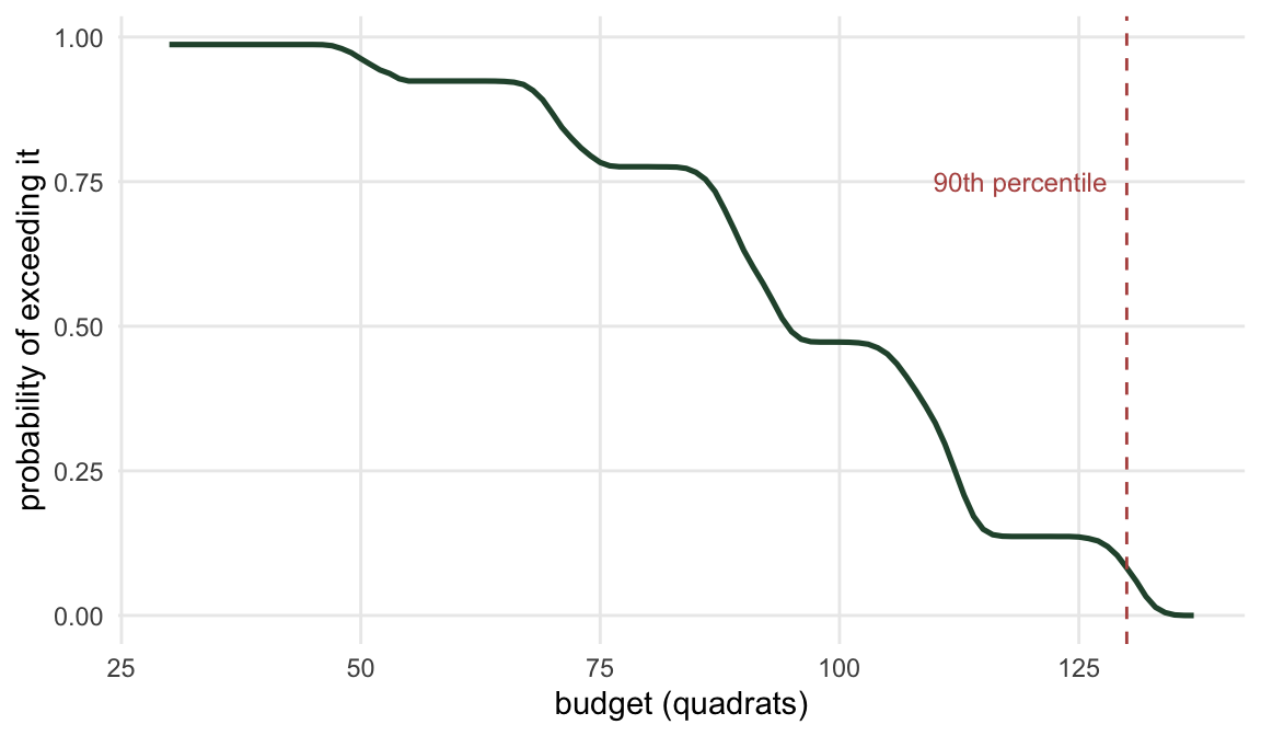
A crew that planned for `r n1` quadrats will visit more than 80 in `r sprintf("%.0f%%", 100 * p80)` of seasons and more than 120 in `r sprintf("%.0f%%", 100 * p120)`. The ninetieth percentile is `r q90` quadrats, roughly `r sprintf("%.1f", q90 / n1)` times the initial sample. Budget from that, not from the mean.
```{r}
#| label: fig-budget
#| echo: false
#| fig-cap: "Probability that the adaptive sample exceeds a given number of quadrats, from 20,000 simulated seasons. The dashed line marks the ninetieth percentile, a safer planning figure than the mean."
#| fig-alt: "A falling curve showing the probability of exceeding a budget, starting near one at 30 quadrats and dropping towards zero by about 137, with a dashed vertical line at the ninetieth percentile of 130."
#| fig-width: 6.0
#| fig-height: 3.5
bs <- seq(min(nf), max(nf), by = 1)
ex <- data.frame(budget = bs, p = sapply(bs, function(b) mean(nf > b)))
ggplot(ex, aes(budget, p)) +
geom_line(colour = "#275139", linewidth = 0.9) +
geom_vline(xintercept = q90, linetype = 2, colour = "#b5534e") +
annotate("text", x = q90 - 2, y = 0.75, label = "90th percentile",
hjust = 1, size = 3.2, colour = "#b5534e") +
labs(x = "budget (quadrats)", y = "probability of exceeding it") +
theme_minimal(base_size = 11) + te_canvas + theme(panel.grid.minor = element_blank())
```
If the tail is unaffordable, the standard remedies are a smaller initial sample, a stricter condition, or a hard cap on expansion. A cap breaks the unbiasedness of the estimators, so it needs its own treatment rather than a quiet truncation in the field.
## Check 3: is each network counted once?
The Horvitz-Thompson estimator sums over the **distinct** networks the initial sample touched. If two initial units land in the same cluster, that cluster still enters once. Dropping the `unique()` is a one-word slip that looks harmless and is not.
```{r}
#| label: double-count
#| echo: true
ht_double <- function(pop, nets, n1, B, seed) {          # WRONG on purpose
  set.seed(seed); N <- pop$N; est <- numeric(B)
  for (b in 1:B) {
    init <- sample.int(N, n1)
    hit  <- nets$net_id[init]                            # no unique(): repeats
    a <- 1 - choose2(N - nets$m[hit], n1) / choose2(N, n1)
    est[b] <- sum(nets$tot[hit] / a) / N
  }
  est
}
wrong <- ht_double(pop, nets, n1, 20000L, 202L)
set.seed(202); right <- numeric(20000L)
for (b in 1:20000L) right[b] <- acs_draw(pop, nets, n1)$ht
c(truth = round(mu, 4), correct = round(mean(right), 4),
  double_counted = round(mean(wrong), 4))
```
```{r}
#| label: dc-nums
#| include: false
dc_bias <- mean(wrong) - mu; dc_pct <- 100 * dc_bias / mu
```
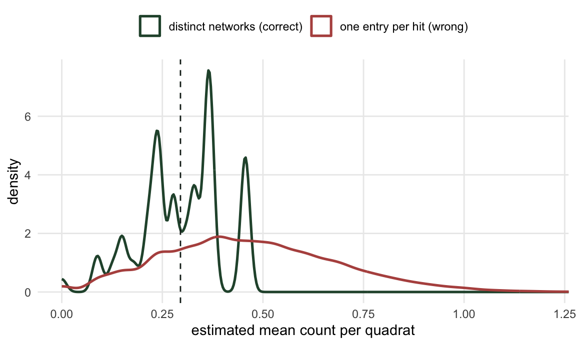
The correct estimator lands on `r sprintf("%.4f", mean(right))` against a truth of `r sprintf("%.4f", mu)`. The version that counts a network once per initial hit gives `r sprintf("%.4f", mean(wrong))`, a bias of `r sprintf("%+.0f%%", dc_pct)`. It fails in the same direction as the naive mean from the first post, and for the same reason: clusters are what the initial sample hits repeatedly, so counting the hits over-weights the clusters.
```{r}
#| label: fig-double-count
#| echo: false
#| fig-cap: "Sampling distributions of the correct and the double-counting estimator over 20,000 draws. The slip moves the whole distribution off the truth and spreads it much wider as well."
#| fig-alt: "Two density curves. The correct estimator is centred on the dashed true-mean line while the double-counting version sits well to the right of it and is far wider, with a long right tail."
#| fig-width: 6.0
#| fig-height: 3.6
dd <- rbind(data.frame(est = right, which = "distinct networks (correct)"),
data.frame(est = wrong, which = "one entry per hit (wrong)"))
ggplot(dd, aes(est, colour = which)) +
geom_density(linewidth = 0.9) +
geom_vline(xintercept = mu, linetype = 2, colour = "#16241d") +
scale_colour_manual(values = c("distinct networks (correct)" = "#275139",
"one entry per hit (wrong)" = "#b5534e"), name = NULL) +
coord_cartesian(xlim = c(0, 1.2)) +
labs(x = "estimated mean count per quadrat", y = "density") +
theme_minimal(base_size = 11) + te_canvas +
theme(legend.position = "top", panel.grid.minor = element_blank())
```
The check that catches it needs no theory: simulate from a population you made yourself, run your estimator over many draws, and confirm the average lands on the value you put in. A bias of `r sprintf("%.0f%%", dc_pct)` is obvious in that test and invisible in a single field data set.
## The short version
Sweep the condition and read the standard error, not only the efficiency. Budget from the upper tail of the sample size, not the mean. And test your estimator against a known truth before it ever sees real counts. None of the three needs field data, and each of them costs a few minutes.
## References
Thompson SK 1990 J Am Stat Assoc 85(412):1050-1059 (10.1080/01621459.1990.10474975)
Thompson SK 1991 Biometrics 47(3):1103-1115 (10.2307/2532662)
Brown JA 2003 Environ Ecol Stat 10(1):95-105 (10.1023/A:1021933424344)
Turk P, Borkowski JJ 2005 Environ Ecol Stat 12(1):55-94 (10.1007/s10651-005-6818-0)
Thompson SK, Seber GAF 1996 Adaptive Sampling. Wiley (ISBN 978-0-471-55871-2)
## Related tutorials
- [Adaptive cluster sampling in R](../adaptive-cluster-sampling/)
- [Horvitz-Thompson for adaptive samples](../horvitz-thompson-for-adaptive-samples/)
- [When does adaptive sampling pay?](../when-does-adaptive-sampling-pay/)
- [Checking a survey design](../checking-a-survey-design/)