library(ggplot2); library(MASS)
theme_te <- function() {
  theme_minimal(base_size = 12) +
    theme(
          plot.background  = element_rect(fill = "#f5f4ee", colour = NA),
          panel.background = element_rect(fill = "#f5f4ee", colour = NA),
          panel.grid.minor = element_blank(),
          panel.grid.major = element_line(colour = "#e7e6da", linewidth = 0.3),
          plot.title = element_text(colour = "#16241d", face = "bold", size = 13),
          plot.subtitle = element_text(colour = "#5d6b61", size = 10),
          axis.title = element_text(colour = "#46604a"),
          axis.text = element_text(colour = "#5d6b61"),
          legend.title = element_text(colour = "#46604a"),
          legend.text = element_text(colour = "#5d6b61"))
}
pal_forest <- "#275139"; pal_gold <- "#cda23f"; pal_rust <- "#b5534e"

grts_address <- function(x, y, L = 8L) {
  n <- length(x); addr <- numeric(n)
  recurse <- function(idx, xlo, xhi, ylo, yhi, level, prefix) {
    if (level >= L || length(idx) <= 1L) { addr[idx] <<- prefix * 4^(L - level); return(invisible(NULL)) }
    xm <- (xlo + xhi)/2; ym <- (ylo + yhi)/2
    q <- (x[idx] >= xm) + 2L*(y[idx] >= ym); perm <- sample(0:3)
    for (qq in 0:3) {
      sub <- idx[q == qq]; if (length(sub) == 0L) next
      cxlo <- if (qq %% 2L == 1L) xm else xlo; cxhi <- if (qq %% 2L == 1L) xhi else xm
      cylo <- if (qq >= 2L) ym else ylo;       cyhi <- if (qq >= 2L) yhi else ym
      recurse(sub, cxlo, cxhi, cylo, cyhi, level + 1L, prefix*4 + perm[qq + 1L])
    }
  }
  recurse(seq_len(n), 0, 1, 0, 1, 0L, 0); addr
}
grts_draw <- function(x, y, m, pip = NULL, L = 8L) {
  n <- length(x); if (is.null(pip)) pip <- rep(m/n, n)
  a <- grts_address(x, y, L); ord <- order(a, runif(n))
  cs <- cumsum(pip[ord]); picks <- runif(1) + 0:(m - 1)
  ord[findInterval(picks, c(0, cs), rightmost.closed = TRUE)]
}Checking a survey design
R
survey design
model diagnostics
monitoring
ecology tutorial
Three diagnostics for a spatially balanced ecological survey in R: realised inclusion probabilities, systematic grid aliasing, and what the frame leaves out.
Corrected 7 October 2026: the post said GRTS is never much worse than a systematic grid, a claim drawn from a single smooth landscape; it now says that on smooth ground a grid can beat GRTS, by a margin that varies from one landscape to the next.
Corrected 30 September 2026: on the smooth landscape the post said GRTS was modestly ahead of the systematic grid, but the variance ratio it quoted is grid over GRTS and below one, so it now says the grid is modestly ahead.
The three previous posts built a spatially balanced design, measured what it buys, and showed how to weight when the inclusion probabilities are unequal. This one asks what can still go wrong. Survey design is unusual among the topics on this blog in that the assumptions are mostly under your control: you chose the frame, you set the inclusion probabilities, you decided how the sites are laid out. That makes the failures administrative rather than statistical, and administrative failures are quiet. Three checks are worth running before a monitoring programme goes to the field, and the third one cannot be run at all after the fact.
Check one: do the realised inclusion probabilities match the plan?
Everything downstream rests on pi_i. The Horvitz-Thompson weights are the reciprocals of the numbers you wrote down, so if the draw does not actually select units at those rates, the weighting corrects for a design that never happened. This is worth verifying because it is easy to break: capping probabilities at one, renormalising after the cap, dropping units from the frame, or a bug in the size measure all shift the realised rates away from the intended ones.
The check is a simulation of your own design. Run the draw many times against the frame you plan to use, count how often each unit is selected, and compare with the intended probabilities.
set.seed(404)
side <- 22
g <- expand.grid(x = seq(0.02, 0.98, length.out = side),
                 y = seq(0.02, 0.98, length.out = side))
N <- nrow(g); m <- 40
w <- 1 + 3 * g$x                                   # intended density rises to the east
pip <- m * w / sum(w); pip <- pmin(pip, 0.999); pip <- m * pip / sum(pip)

set.seed(111)
R <- 6000
counts <- integer(N)
for (r in seq_len(R)) { s <- grts_draw(g$x, g$y, m, pip = pip); counts[s] <- counts[s] + 1L }
pi_emp <- counts / R
cor_pi <- cor(pi_emp, pip); dev_pi <- max(abs(pi_emp - pip))
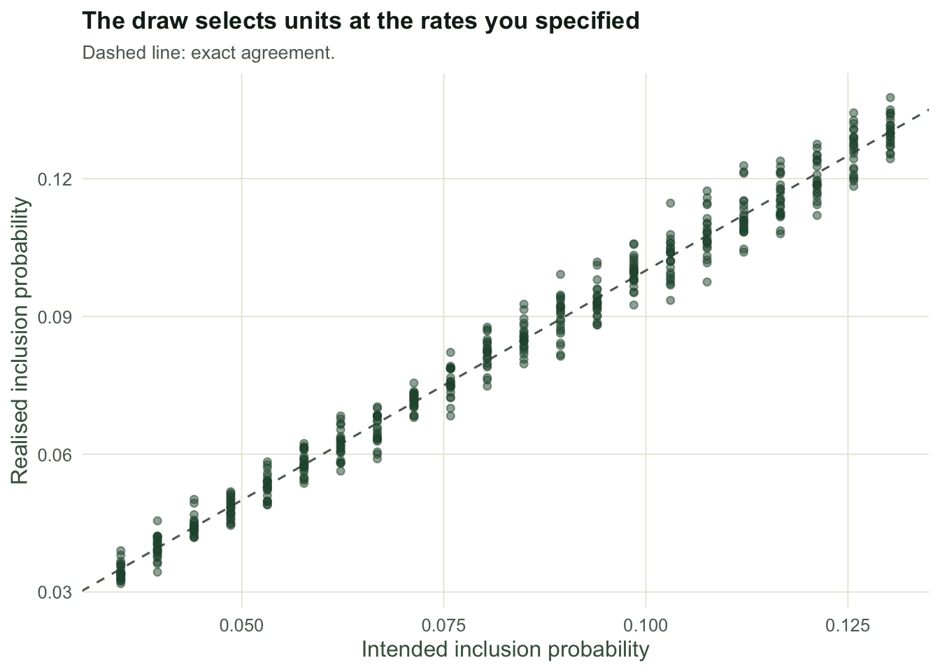
Over 6000 draws the realised and intended inclusion probabilities correlate at 0.9927, with a largest absolute deviation of 0.0112, comfortably inside Monte Carlo error for this many replicates. The design does what the specification says. A failed version of this check looks obvious: a systematic gap between the two, or a set of units pinned at zero because they fell out of the frame.
Check two: would a systematic grid have aliased?
A regular grid is the other way to guarantee even spatial coverage, and it is tempting because it is simple to explain and simple to navigate to. Its weakness is that it has almost no randomisation left: a grid with a random start has only as many distinct configurations as there are offsets. If the landscape carries periodic structure at the grid spacing, every site lands at the same phase of the cycle, and the sample tells you about that phase and nothing else. The estimate stays roughly unbiased across random starts, but its variance explodes.
Periodic structure in ecology is not exotic. Agricultural furrows, planted rows, dune and swale systems, ridge and slack, drainage ditches and terraces all impose regular spacing on a landscape.
sideF <- 30
gf <- expand.grid(r = 1:sideF, c = 1:sideF)
gf$x <- (gf$c - 0.5)/sideF; gf$y <- (gf$r - 0.5)/sideF
Nf <- nrow(gf); step <- sideF/6; base_rows <- seq(1, sideF, by = step)

set.seed(707)
per <- 6                                          # waves match the grid spacing
y_per <- 10 + 3*sin(2*pi*per*gf$x) + rnorm(Nf, 0, 0.5)
Dmf <- as.matrix(dist(cbind(gf$x, gf$y)))
set.seed(909)
y_smooth <- as.numeric(mvrnorm(1, rep(10, Nf), 3*exp(-Dmf/0.2)))

sys_sample <- function(off) {
  rr <- ((base_rows - 1 + off[1]) %% sideF) + 1
  cc <- ((base_rows - 1 + off[2]) %% sideF) + 1
  which(gf$r %in% rr & gf$c %in% cc)
}

set.seed(808)
Rr <- 3000
sys_per <- numeric(Rr); grts_per <- numeric(Rr)
sys_sm  <- numeric(Rr); grts_sm  <- numeric(Rr)
for (k in seq_len(Rr)) {
  ss <- sys_sample(sample(0:(step - 1), 2, replace = TRUE))
  sg <- grts_draw(gf$x, gf$y, length(ss))
  sys_per[k] <- mean(y_per[ss]);    grts_per[k] <- mean(y_per[sg])
  sys_sm[k]  <- mean(y_smooth[ss]); grts_sm[k]  <- mean(y_smooth[sg])
}
ratio_per <- var(sys_per) / var(grts_per)
ratio_sm  <- var(sys_sm)  / var(grts_sm)
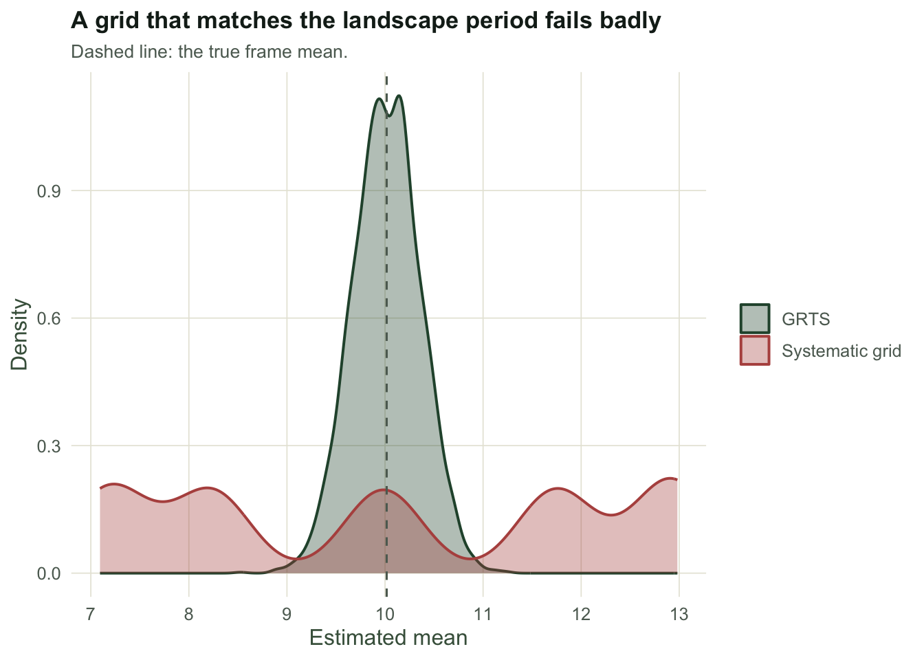
On the periodic landscape the systematic grid has 40 times the variance of GRTS at the same sample size: standard deviation 2.153 against 0.340. Any single systematic survey returns a confident, precise-looking number that is a property of the phase it happened to land on. On the smooth landscape, where no periodicity exists to lock onto, the two designs are comparable and the grid is modestly ahead, with a variance ratio (grid over GRTS) of 0.91.
The asymmetry is the point. On smooth ground a grid can beat GRTS, by a margin that varies from one landscape to the next, but GRTS is enormously better in the case that ruins a grid, and you do not need to know in advance whether your landscape has periodic structure at your spacing. That is what the randomised hierarchy is protecting you from.
Check three: what did the frame leave out?
The first two checks can be run from your desk. This one cannot be run from the data at all, and it is the one that most often decides whether a monitoring programme means what its report says.
A design-based estimate is unbiased for the frame. If places were quietly dropped because they are steep, private, far from a road or under water at the time of the survey, then the frame is a biased subset of the population, and every standard error you compute is honest about sampling error while silent about the omission.
set.seed(707)
Dm <- as.matrix(dist(g))
elev <- 0.6*g$x + 0.8*g$y                          # ground rises to the north-east
z <- 8 + 5*elev + as.numeric(mvrnorm(1, rep(0, N), 1.5*exp(-Dm/0.2)))
access <- elev < quantile(elev, 0.82)              # the high corner is never surveyed
mu_pop <- mean(z); mu_frame <- mean(z[access])

set.seed(808)
idx <- which(access)
est <- replicate(3000, mean(z[idx[grts_draw(g$x[idx], g$y[idx], m)]]))
err_frame <- mean(est) - mu_frame
err_pop   <- mean(est) - mu_pop
se_design <- sd(est)
n_se <- abs(err_pop) / se_design
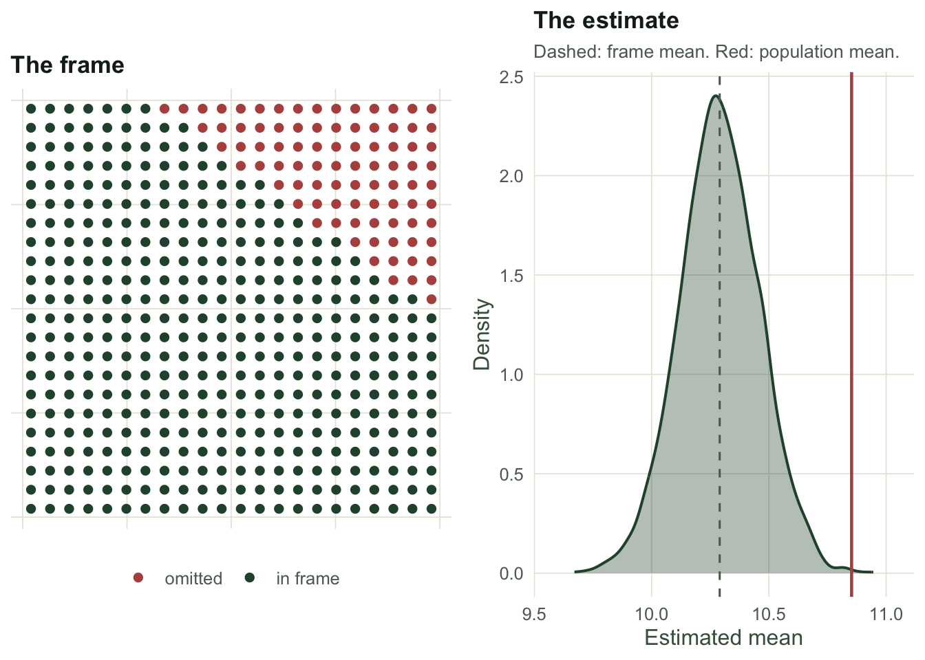
The frame covers 82% of the landscape, leaving out the highest fifth of the ground. Against the frame mean the design is exactly as advertised: average error -0.001. Against the population mean it is off by -0.563, which is 4.3 design standard errors. No diagnostic run on the sample can see this, because every sampled unit is a legitimate member of the frame and the estimator is behaving correctly. The error lives in the gap between the list you sampled and the population you are going to write about.
What the checks can and cannot settle
The first two checks are genuine tests with a possible failure: the realised probabilities can disagree with the plan, and a grid can alias. Run them before the field season, when the answer can still change the design.
The third is not a test. It is a statement you have to write down and defend, because the data will never contradict it. The useful discipline is to record what the frame excludes and why, and to say plainly whether the reported quantity is a property of the surveyed population or of the accessible part of it. A design-based survey gives you an unusually clean guarantee, and the guarantee is precisely as wide as the frame.
References
Stevens DL, Olsen AR 2004 Journal of the American Statistical Association 99(465):262-278 (10.1198/016214504000000250)
Stevens DL, Olsen AR 2003 Environmetrics 14(6):593-610 (10.1002/env.606)
Olsen AR, Sedransk J, Edwards D, Gotway CA, Liggett W, Rathbun S, Reckhow KH, Young LJ 1999 Environmental Monitoring and Assessment 54(1):1-45 (10.1023/A:1005823911258)
Theobald DM, Stevens DL, White D, Urquhart NS, Olsen AR, Norman JB 2007 Environmental Management 40(1):134-146 (10.1007/s00267-005-0199-x)