library(ggplot2)
library(MASS)

theme_te <- function() {
  theme_minimal(base_size = 12) +
    theme(
          plot.background  = element_rect(fill = "#f5f4ee", colour = NA),
          panel.background = element_rect(fill = "#f5f4ee", colour = NA),
          panel.grid.minor = element_blank(),
          panel.grid.major = element_line(colour = "#e7e6da", linewidth = 0.3),
          plot.title = element_text(colour = "#16241d", face = "bold", size = 13),
          plot.subtitle = element_text(colour = "#5d6b61", size = 10),
          axis.title = element_text(colour = "#46604a"),
          axis.text = element_text(colour = "#5d6b61"),
          legend.title = element_text(colour = "#46604a"),
          legend.text = element_text(colour = "#5d6b61"),
          strip.text = element_text(colour = "#16241d", face = "bold"))
}
pal_forest <- "#275139"; pal_rust <- "#b5534e"; pal_gold <- "#cda23f"Spatially balanced sampling with GRTS
R
survey design
spatial statistics
monitoring
ecology tutorial
Design-based sampling for ecological monitoring: the Horvitz-Thompson estimator, and GRTS from scratch in R to spread survey sites evenly across a landscape.
Corrected 8 October 2026: the post said that any leading part of the reordered sample is itself balanced and that sites can be dropped from the tail without losing the spread; it now says a leading part stays fairly spread out but that, when the sample size is not a power of four, the first few sites can still bunch. It also said a regular grid is not randomised; it now says a grid leaves at most its starting point to chance.
Corrected 1 October 2026: the code reordered the selected sites by reversing their spatial address digits, which leaves them in an effectively random order and does not keep the leading sites spread out; it now reverses the base-four digits of each site’s position in the address order, as the reverse-hierarchical ordering of GRTS does.
Most of the statistics on this blog treat the data as fixed and the sampling as given, then model the process that generated the numbers. Survey sampling turns that around. Here the population is a fixed set of places (a lake, a set of stream reaches, every 1 km cell in a park), and the only thing that is random is which places you decide to visit. That single choice, the sampling design, carries the whole inferential weight. Get it right and you can estimate a regional mean or total with an honest error bound and no model of nature at all. Get it wrong and no clever analysis afterwards repairs it.
This post is the first of a short series on design-based inference for ecological monitoring, and on the workhorse of modern environmental surveys: the Generalised Random Tessellation Stratified design, or GRTS. We build it from scratch so the mechanism is visible, then measure the one thing it is meant to deliver: a sample that is spread evenly across space.
The frame and the Horvitz-Thompson estimator
A design-based survey starts with a sampling frame: an explicit list of every unit that could be sampled. For a set of survey plots that is just their coordinates. Each unit i is assigned an inclusion probability pi_i, the probability that the design selects it. The frame and the inclusion probabilities are the whole model. There is no assumption that the resource follows any distribution.
Given a sample s, the Horvitz-Thompson estimator of a total is a weighted sum, where each sampled value is divided by its inclusion probability:
\[\hat{t}_{HT} = \sum_{i \in s} \frac{y_i}{\pi_i}.\]
The division by pi_i is the key. A unit that was unlikely to be selected stands in for many similar unselected units, so it gets a large weight. For equal-probability sampling of m units from N, every pi_i equals m/N, and the estimated mean collapses to the plain sample mean. As soon as the probabilities differ, the plain mean is biased whenever the values are related to the probabilities, and the Horvitz-Thompson form is the one that stays unbiased. The next posts lean on that fact; here everything is equal-probability, so the sample mean is enough.
Why not just scatter points at random?
Simple random sampling gives every unit the same inclusion probability and is unbiased. Its weakness is spatial. Ecological resources are autocorrelated: neighbouring places resemble each other. A simple random sample of a small number of sites leaves clumps in some parts of the landscape and holes in others, and the clumped sites carry redundant information while the holes carry none.
set.seed(4301)
side <- 20
frame <- expand.grid(x = seq(0.025, 0.975, length.out = side),
                     y = seq(0.025, 0.975, length.out = side))
N <- nrow(frame)
frame$x <- frame$x + runif(N, -0.018, 0.018)
frame$y <- frame$y + runif(N, -0.018, 0.018)
m <- 30
set.seed(4302)
srs <- sample(N, m)
A regular grid fixes the spacing problem but leaves at most its starting point to chance, and we will see in the checking post that a rigid grid can fail badly on periodic landscapes. GRTS threads the needle: it draws a random sample whose inclusion probabilities you control exactly, yet forces that sample to be spread out.
GRTS from scratch
The idea has three moving parts. First, impose a hierarchy of nested quadrants on the study region and give every unit an address that records which quadrant it falls in at each level, with the four quadrant labels shuffled independently at every node. Units that share the same coarse quadrant share the leading digits of their address, so the address is a space-filling ordering: walk along it and you finish each quadrant, at every level, before you move to the next, although the step from one quadrant to the next can jump across the map. Second, lay the inclusion probabilities along that ordering and take a systematic sample of it with a random start. Because the ordering is space-filling, a systematic pick is automatically spread across the map. Third, reorder the selected sites by reversing the base-four digits of their position in the address order, so that a leading part of the ordered sample stays fairly spread out and you can drop sites from the tail while keeping much of the spread; when the sample size is not a power of four, as here, this works only roughly and the first few sites can still bunch.
The address is a short recursion. At each node we split the box into four, read off which quadrant every point is in, shuffle the four labels, and descend.
grts_address <- function(x, y, L = 8L) {
  n <- length(x); addr <- numeric(n)
  recurse <- function(idx, xlo, xhi, ylo, yhi, level, prefix) {
    if (level >= L || length(idx) <= 1L) {       # pad a short address out to full depth,
      addr[idx] <<- prefix * 4^(L - level)       # so all addresses sort on the same scale
      return(invisible(NULL))
    }
    xm <- (xlo + xhi) / 2; ym <- (ylo + yhi) / 2
    q <- (x[idx] >= xm) + 2L * (y[idx] >= ym)   # 0 SW, 1 SE, 2 NW, 3 NE
    perm <- sample(0:3)                          # shuffle labels at this node
    for (qq in 0:3) {
      sub <- idx[q == qq]; if (length(sub) == 0L) next
      cxlo <- if (qq %% 2L == 1L) xm else xlo; cxhi <- if (qq %% 2L == 1L) xhi else xm
      cylo <- if (qq >= 2L) ym else ylo;       cyhi <- if (qq >= 2L) yhi else ym
      recurse(sub, cxlo, cxhi, cylo, cyhi, level + 1L, prefix * 4 + perm[qq + 1L])
    }
  }
  recurse(seq_len(n), 0, 1, 0, 1, 0L, 0)
  addr
}
The draw itself puts the inclusion probabilities in address order, forms their cumulative sum, and selects the units whose intervals contain m equally spaced points offset by a random start. With every pi_i equal to m/N, the intervals all have the same length and the total length is m, so exactly m distinct units are chosen. The reverse-hierarchical reordering closes it out.
grts_draw <- function(x, y, m, pip = NULL, L = 8L) {
  n <- length(x)
  if (is.null(pip)) pip <- rep(m / n, n)
  a <- grts_address(x, y, L)
  ord <- order(a, runif(n))                      # random tie-break within a cell
  cs <- cumsum(pip[ord])
  picks <- runif(1) + 0:(m - 1)                  # systematic points, random start
  sel <- ord[findInterval(picks, c(0, cs), rightmost.closed = TRUE)]
  rev4 <- function(v, L) { r <- numeric(length(v)); vv <- v
    for (k in seq_len(L)) { r <- r * 4 + vv %% 4; vv <- vv %/% 4 }; r }
  nd <- max(1L, ceiling(log(length(sel), 4)))     # sel is in address order: reverse
  sel[order(rev4(seq_along(sel) - 1, nd), runif(length(sel)))]  # each position's digits
}

set.seed(4303)
grts <- grts_draw(frame$x, frame$y, m)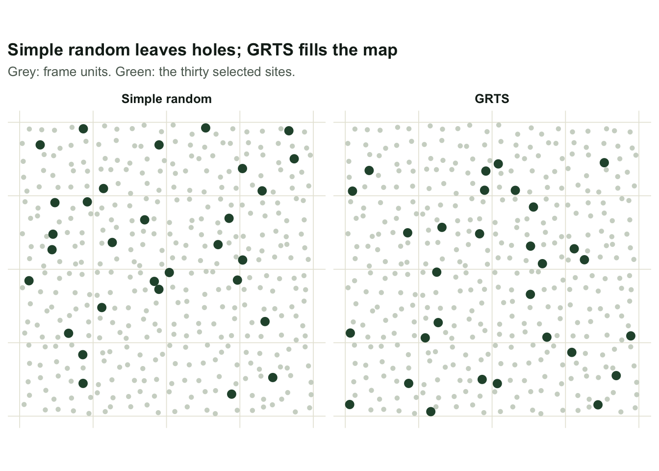
Measuring the spread
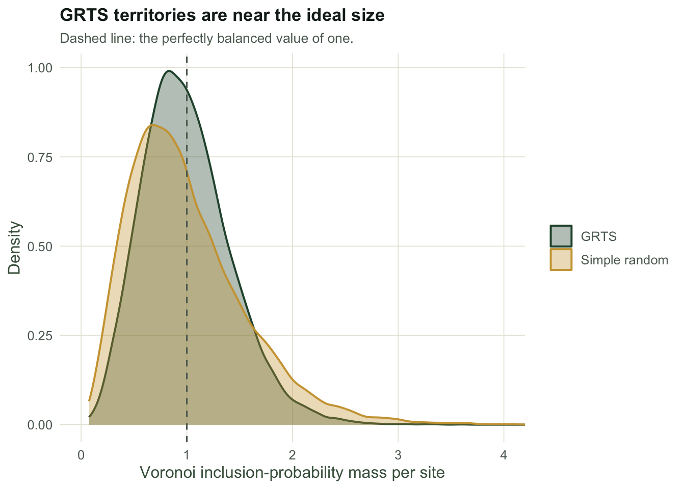
“Evenly spread” needs a number. A clean one is the Voronoi inclusion-probability mass. Assign every frame unit to its nearest sampled site, then add up the inclusion probabilities in each site’s territory. If the sample were perfectly balanced, each territory would hold the same probability mass, exactly one. The variance of those masses across sites measures the imbalance: zero is perfect, larger is worse.
balance <- function(x, y, sel, pip = NULL) {
  n <- length(x); if (is.null(pip)) pip <- rep(length(sel) / n, n)
  nn <- max.col(-as.matrix(dist(rbind(cbind(x[sel], y[sel]),
                                      cbind(x, y))))[-(seq_along(sel)),
                                      seq_along(sel)], ties.method = "first")
  mass <- tapply(pip, factor(nn, levels = seq_along(sel)), sum); mass[is.na(mass)] <- 0
  var(as.numeric(mass))
}

set.seed(4304)
bal_grts <- mean(replicate(400, balance(frame$x, frame$y, grts_draw(frame$x, frame$y, m))))
bal_srs  <- mean(replicate(400, balance(frame$x, frame$y, sample(N, m))))
ratio_bal <- bal_srs / bal_grts
Averaged over 400 draws each, the imbalance is 0.308 for simple random sampling and 0.107 for GRTS, a factor of 2.89 less variance in the mass a GRTS site has to cover. GRTS is doing exactly what it promised: same landscape, same sample size, a far more even reach.
What GRTS gives you, and what it does not
GRTS is a randomised design whose inclusion probabilities you set exactly (all equal in this post), and whose sample is spread across the landscape. That combination is why it underpins large national programmes for streams, lakes, wetlands and forests. What it does not do on its own is tell you how precise your estimate is: the spread buys real precision, but reading that precision off correctly needs a variance estimator that knows about the spatial structure, which is the subject of the next post. And no design rescues a frame that leaves places out with nothing to link them back: a resource that is neither listed nor tied to a listed unit can never be sampled, however cleverly. If the design attaches each unlisted resource to a listed one by a stated rule, the unlisted resource inherits a known, non-zero inclusion probability through the unit it is attached to, and it can enter the sample after all; what cannot be rescued is a gap that no rule reaches, because that is a property of the frame rather than of the draw.
References
Horvitz DG, Thompson DJ 1952 Journal of the American Statistical Association 47(260):663-685 (10.1080/01621459.1952.10483446)
Stevens DL, Olsen AR 2004 Journal of the American Statistical Association 99(465):262-278 (10.1198/016214504000000250)
Stevens DL 1997 Environmetrics 8(3):167-195 (10.1002/(SICI)1099-095X(199705)8:3<167::AID-ENV239>3.0.CO;2-D)
Theobald DM, Stevens DL, White D, Urquhart NS, Olsen AR, Norman JB 2007 Environmental Management 40(1):134-146 (10.1007/s00267-005-0199-x)