library(ggplot2); library(MASS)
theme_te <- function() {
  theme_minimal(base_size = 12) +
    theme(
          plot.background  = element_rect(fill = "#f5f4ee", colour = NA),
          panel.background = element_rect(fill = "#f5f4ee", colour = NA),
          panel.grid.minor = element_blank(),
          panel.grid.major = element_line(colour = "#e7e6da", linewidth = 0.3),
          plot.title = element_text(colour = "#16241d", face = "bold", size = 13),
          plot.subtitle = element_text(colour = "#5d6b61", size = 10),
          axis.title = element_text(colour = "#46604a"),
          axis.text = element_text(colour = "#5d6b61"),
          legend.title = element_text(colour = "#46604a"),
          legend.text = element_text(colour = "#5d6b61"))
}
pal_forest <- "#275139"; pal_gold <- "#cda23f"; pal_rust <- "#b5534e"

# GRTS engine (see the opener for the derivation); returns sites in spatial order
grts_address <- function(x, y, L = 8L) {
  n <- length(x); addr <- numeric(n)
  recurse <- function(idx, xlo, xhi, ylo, yhi, level, prefix) {
    if (level >= L || length(idx) <= 1L) { addr[idx] <<- prefix * 4^(L - level); return(invisible(NULL)) }
    xm <- (xlo + xhi) / 2; ym <- (ylo + yhi) / 2
    q <- (x[idx] >= xm) + 2L * (y[idx] >= ym); perm <- sample(0:3)
    for (qq in 0:3) {
      sub <- idx[q == qq]; if (length(sub) == 0L) next
      cxlo <- if (qq %% 2L == 1L) xm else xlo; cxhi <- if (qq %% 2L == 1L) xhi else xm
      cylo <- if (qq >= 2L) ym else ylo;       cyhi <- if (qq >= 2L) yhi else ym
      recurse(sub, cxlo, cxhi, cylo, cyhi, level + 1L, prefix * 4 + perm[qq + 1L])
    }
  }
  recurse(seq_len(n), 0, 1, 0, 1, 0L, 0); addr
}
grts_draw <- function(x, y, m, L = 8L) {          # returns sites in ascending address order
  n <- length(x); pip <- rep(m / n, n)
  a <- grts_address(x, y, L); ord <- order(a, runif(n))
  cs <- cumsum(pip[ord]); picks <- runif(1) + 0:(m - 1)
  sort_sel <- ord[findInterval(picks, c(0, cs), rightmost.closed = TRUE)]
  sort_sel[order(a[sort_sel])]
}

set.seed(101)
side <- 22
frame <- expand.grid(x = seq(0.02, 0.98, length.out = side),
                     y = seq(0.02, 0.98, length.out = side))
N <- nrow(frame)
Dm <- as.matrix(dist(frame)); rho <- 0.18
z <- as.numeric(mvrnorm(1, rep(10, N), 4 * exp(-Dm / rho)))
mu_true <- mean(z)
m <- 40
f <- m / NDesign-based variance and spatial balance
R
survey design
spatial statistics
monitoring
ecology tutorial
A spatially balanced survey is more precise, but the textbook variance formula does not know it. Estimating design-based variance for GRTS samples in R.
Corrected 14 October 2026: the text said without qualification that the simple-random formula is not biased downward for a GRTS sample and that reporting a survey with it is honest but pessimistic, and that consecutive sites in the GRTS order are neighbours on the map; it now limits the first two to an autocorrelated resource like this one and says consecutive sites tend to lie close together on the map.
Corrected 30 September 2026: the text called both variance estimators upper bounds on the true GRTS variance; it now says they exceed it on average on this landscape, without a guarantee in general.
The previous post built GRTS and showed that it spreads survey sites evenly across a landscape. Spread is not the goal in itself; the goal is a more precise estimate of whatever you went out to measure. This post makes that precision concrete, and then delivers the catch that trips up most first-time users of spatially balanced designs: the standard variance formula you were taught for simple random sampling reports the precision you would have had from a random sample, not the precision you actually achieved. You leave the efficiency gain on the table at the reporting stage unless the variance estimator knows about the spatial structure.
A landscape and a target
We work on a fixed frame with a spatially autocorrelated resource, generated once from a Gaussian field with an exponential covariance. Because this is design-based inference, the resource is a fixed set of numbers; the only randomness is the sample. The quantity we estimate is the plain frame mean.
The precision GRTS buys
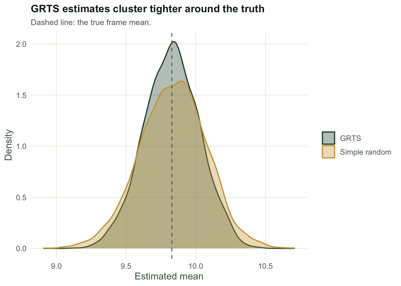
We draw the mean many times under each design and look at the spread of the estimates. This is the design-based sampling distribution: repeat the sampling, hold the resource fixed.
set.seed(202)
R <- 3000
est_srs  <- numeric(R); est_grts <- numeric(R)
for (r in seq_len(R)) {
  est_srs[r]  <- mean(z[sample(N, m)])
  est_grts[r] <- mean(z[grts_draw(frame$x, frame$y, m)])
}
var_srs  <- var(est_srs); var_grts <- var(est_grts)
gain <- var_srs / var_grts
bias_srs  <- mean(est_srs)  - mu_true
bias_grts <- mean(est_grts) - mu_true
Both designs are unbiased: the mean of the estimates is +0.0076 off the truth for simple random and -0.0027 for GRTS, both effectively zero. The difference is in the spread. The variance of the estimated mean is 0.0570 under simple random sampling and 0.0339 under GRTS, so GRTS is 1.68 times more efficient here. On an autocorrelated resource, spreading the sample is worth real precision, and the more autocorrelated the resource, the larger the gain.
The catch: the textbook formula does not know
Here is the part that surprises people. You have a single GRTS sample and want a standard error. The formula every field course teaches is the simple-random one, (1 - f) s^2 / m, where s^2 is the sample variance and f the sampling fraction. Applied to a GRTS sample from an autocorrelated resource like this one, it is not wrong in the sense of being biased downward; it is wrong in the sense of being far too large. It computes the variance you would have had if the sample had been scattered at random, ignoring that GRTS deliberately spread it out.
srs_var_mean <- function(zs) (1 - f) * var(zs) / m
set.seed(303)
v_srs_on_grts <- numeric(2000)
for (r in seq_len(2000)) v_srs_on_grts[r] <- srs_var_mean(z[grts_draw(frame$x, frame$y, m)])
srs_est <- mean(v_srs_on_grts)
srs_ratio <- srs_est / var_grts
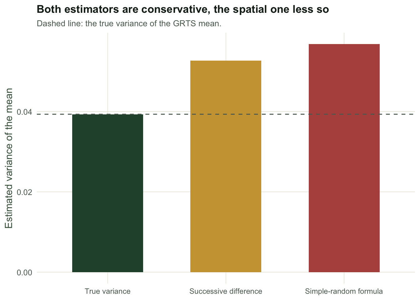
The simple-random formula, averaged over GRTS samples, reports a variance of 0.0568, which is 1.67 times the true GRTS variance of 0.0339. Your confidence interval comes out honest but roughly 29% too wide. The gain in precision is real, but you never see it in the report.
Using the spatial order
The GRTS sample arrives already ordered along the space-filling curve, so neighbouring entries in the list tend to lie close together on the map. That suggests a successive-difference estimator: instead of the overall sample variance, use the squared differences between consecutive sites along the spatial order, which reflect the local variation the balanced design actually leaves behind.
sd_var_mean <- function(zo) (1 - f) / m * sum(diff(zo)^2) / (2 * (m - 1))
set.seed(404)
v_sd <- numeric(2000)
for (r in seq_len(2000)) v_sd[r] <- sd_var_mean(z[grts_draw(frame$x, frame$y, m)])
sd_est <- mean(v_sd)
sd_ratio <- sd_est / var_grts
The successive-difference estimator reports 0.0487, a ratio of 1.44 to the truth. It is closer than the simple-random formula because it uses the spatial ordering, but it still overshoots: averaged over repeated GRTS samples, both estimators exceed the true GRTS variance on this landscape, although neither is guaranteed to be conservative on every resource. That is the honest state of affairs for spatially balanced designs. There is no simple unbiased variance estimator, because the design induces dependence between which sites are chosen that a single sample cannot fully reconstruct.
The honest tool, and the honest limit
The standard estimator for GRTS in practice is the local neighbourhood estimator of Stevens and Olsen (2003). It generalises the successive-difference idea to two dimensions: around each site it forms a small neighbourhood of nearby sites, fits a local mean, and accumulates the local squared residuals with weights that are close to balanced across the sample. It recovers more of the efficiency gain than either estimator here, and it is what the survey software uses, but it too is designed to be near-unbiased or mildly conservative rather than exact.
The lesson is not to distrust the design. GRTS genuinely reduces the variance of your estimate. The lesson is that a spatially balanced sample and a simple-random variance formula are a mismatched pair: the design gives you the precision, and the variance estimator has to be the one that reads it back. If you report a spatially balanced survey of an autocorrelated resource with the textbook standard error, you are likely to be honest but pessimistic, and the more autocorrelated the resource, the more precision you are hiding.
References
Stevens DL, Olsen AR 2003 Environmetrics 14(6):593-610 (10.1002/env.606)
Stevens DL, Olsen AR 2004 Journal of the American Statistical Association 99(465):262-278 (10.1198/016214504000000250)
Horvitz DG, Thompson DJ 1952 Journal of the American Statistical Association 47(260):663-685 (10.1080/01621459.1952.10483446)