library(ggplot2)
library(patchwork)

te_paper  <- "#f5f4ee"
te_ink    <- "#16241d"
te_body   <- "#2c3a31"
te_forest <- "#275139"
te_rust   <- "#b5534e"
te_gold   <- "#c9b458"
te_line   <- "#dad9ca"

theme_datasheet <- function() {
  theme_minimal(base_size = 12) +
    theme(plot.background  = element_rect(fill = te_paper, colour = NA),
          panel.background = element_rect(fill = te_paper, colour = NA),
          panel.grid.major = element_line(colour = te_line, linewidth = 0.3),
          panel.grid.minor = element_blank(),
          text             = element_text(colour = te_body),
          plot.title       = element_text(colour = te_ink, face = "bold"),
          plot.subtitle    = element_text(colour = te_body),
          axis.text        = element_text(colour = te_body))
}Weighted draws without replacement: sample() in R
R
survey design
sampling
monitoring
reproducibility
ecology tutorial
R’s sample(prob =) without replacement does not select sites at n w / sum(w). What that does to a Horvitz-Thompson mean, and two survey samplers that do.
A monitoring programme covers 400 wetland sites. Eighty of them are fen, the rare class the programme exists for, and the design says fen sites should be twenty times as likely to be visited as the common marsh sites around them. The analyst writes the intended inclusion probabilities as n * w / sum(w), draws the sample of 40 with one line, sample(sites, 40, prob = w), and plans to estimate mean plant species richness per site with a Horvitz-Thompson mean that divides each observation by those intended probabilities. Nothing warns, nothing prints, and a sample of 40 distinct sites comes back.
The help page for sample() says what happens in that line, in one sentence: “If replace is false, these probabilities are applied sequentially, that is the probability of choosing the next item is proportional to the weights amongst the remaining items.” Its See Also section points to the CRAN package sampling “for other methods of weighted sampling without replacement”. So this is not an undocumented trap, and the mechanism is textbook. Successive (or sequential) unequal-probability sampling is catalogued in Brewer and Hanif’s book on sampling with unequal probabilities, and Tille’s Sampling Algorithms treats it alongside the designs that do reach prescribed probabilities; both make the point that the inclusion probabilities of a successive draw are not proportional to the weights. What neither the help page nor the one-liner tells the analyst is how far apart the two sets of probabilities are on a frame an ecologist would build, what that does to the estimate, and which draw to use instead. That is what this post measures.
Three posts on this site sit right next to it. Checking a survey design owns the diagnostic: its check one runs the draw thousands of times, counts how often each unit comes up, and compares with the plan. It demonstrates the check on a design that passes, and it lists the ways a design can fail it: capping probabilities at one, renormalising after the cap, units dropped from the frame, a bug in the size measure. It does not list the sampler, and the sampler is the one failure a careful analyst cannot fix with their own arithmetic. Unequal-probability spatial sampling builds the same kind of oversampled design and concludes, in its section on the biased plain mean, that “the Horvitz-Thompson mean removes exactly that bias”. That is true of the draw it uses, and this post is the footnote the conclusion needs, because it is not true of the one-line draw. Horvitz-Thompson for adaptive samples uses the same estimator with inclusion probabilities derived by hand, correctly, for networks; nothing here changes that.
The post is also a member of a small family on this site about computations that change the answer without saying so. When integrate() in R returns zero and says OK is the numerical case: a base R function doing what its help page describes, silently, in a setting where the documented behaviour costs the estimate. The case below is the design-based one.
The frame and the draw everyone types
The frame is the one described above, and every design constant is fixed here before anything is run: 400 sites, 80 of them in the rare class, richness Poisson with mean 30 in the rare class and 5 elsewhere, weights 20 against 1, and a sample of 40. Six frames are drawn with fresh seeds, so the rare sites land in different places and the richness values differ; the design itself is identical on all six.
n_site  <- 400
n_rare  <- 80
n_draw  <- 40
wt_rare <- 20
wt_comm <- 1
mean_rare <- 30
mean_comm <- 5
n_frame <- 6

make_frame <- function(seed_frame) {
  set.seed(seed_frame)
  is_rare <- rep(FALSE, n_site)
  is_rare[sample.int(n_site, n_rare)] <- TRUE
  rich <- rpois(n_site, ifelse(is_rare, mean_rare, mean_comm))
  wt   <- ifelse(is_rare, wt_rare, wt_comm)
  list(is_rare = is_rare, rich = rich, wt = wt,
       pip = n_draw * wt / sum(wt))
}
frames <- lapply(3000 + seq_len(n_frame), make_frame)

pip_rare <- frames[[1]]$pip[frames[[1]]$is_rare][1]
pip_comm <- frames[[1]]$pip[!frames[[1]]$is_rare][1]
pip_max  <- max(vapply(frames, function(fr) max(fr$pip), 0))
The intended inclusion probability is 0.4167 for a rare site and 0.0208 for a common one. The largest on any frame is 0.417, well below one, so no probability is capped and nothing is renormalised. That matters for the positioning: capping is the named failure mode in the survey-design post, and it plays no part in anything that follows.
What the help page says, and what it costs
With two weight classes the successive draw can be followed exactly. Every rare site is exchangeable with every other rare site, so all that matters after each pick is how many rare sites have already been taken, and the chance that the next pick is rare is the rare sites’ share of the weight that remains. That is a short recursion over the number of rare sites selected, and its expected value at the end, divided by 80, is the exact inclusion probability of a rare site. For a general set of weights no such shortcut exists and the realised probabilities have to be simulated, which is the check-one simulation from the survey-design post; both routes are run here so that each checks the other.
succ_prob_rare <- function(n_pick, n_hi, n_lo, wt_hi, wt_lo) {
  p_k <- c(1, rep(0, n_hi))
  k_hi <- 0:n_hi
  for (j_pick in 0:(n_pick - 1)) {
    k_lo  <- j_pick - k_hi
    valid <- k_lo >= 0 & k_lo <= n_lo
    p_hi  <- ifelse(valid, wt_hi * (n_hi - k_hi) /
                      (wt_hi * (n_hi - k_hi) + wt_lo * (n_lo - k_lo)), 0)
    p_next <- p_k * (1 - p_hi)
    p_next[-1] <- p_next[-1] + (p_k * p_hi)[-(n_hi + 1)]
    p_k <- p_next
  }
  sum(k_hi * p_k) / n_hi
}
pi_rare_exact <- succ_prob_rare(n_draw, n_rare, n_site - n_rare, wt_rare, wt_comm)
pi_comm_exact <- (n_draw - n_rare * pi_rare_exact) / (n_site - n_rare)
ratio_rare_exact <- pi_rare_exact / pip_rare
ratio_comm_exact <- pi_comm_exact / pip_comm

n_mc <- 20000
realised_pi <- function(fr) {
  hits <- integer(n_site)
  rare_count <- integer(n_mc)
  for (r_i in seq_len(n_mc)) {
    picked <- sample.int(n_site, n_draw, prob = fr$wt)
    hits[picked] <- hits[picked] + 1L
    rare_count[r_i] <- sum(fr$is_rare[picked])
  }
  list(pi = hits / n_mc, rare_count = rare_count)
}
set.seed(51)
mc_out <- lapply(frames, realised_pi)
pi_mc  <- lapply(mc_out, function(m) m$pi)
ratio_mc <- t(vapply(seq_len(n_frame), function(i) {
  fr <- frames[[i]]
  c(rare = mean(pi_mc[[i]][fr$is_rare]) / pip_rare,
    comm = mean(pi_mc[[i]][!fr$is_rare]) / pip_comm)
}, numeric(2)))
## the rare-class ratio is the mean rare count per draw over 80, so its
## Monte Carlo error comes from the spread of that count across draws
sd_rare_count <- median(vapply(mc_out, function(m) sd(m$rare_count), 0))
mc_se_rare <- sd_rare_count / (n_rare * sqrt(n_mc)) / pip_rare
A rare site is selected with probability 0.3997 instead of the intended 0.4167, which is 0.959 of the plan, and a common site with probability 0.0251 instead of 0.0208, which is 1.203 of the plan. The simulation agrees: over 20000 draws per frame the rare-class ratio runs from 0.959 to 0.960 across the six frames and the common-class ratio from 1.200 to 1.205. The Monte Carlo standard error of a rare-class ratio is about 0.0005.
The direction is easy to see once the mechanism is spelled out. The first pick uses the weights exactly as written. Each rare site taken removes twenty units of weight from the pool, so the rare class’s share of what remains shrinks faster than its share of the sites, and later picks drift towards the common class. The sample still has 40 sites; it has fewer rare ones and more common ones than the design promised. The expected count of rare sites is 31.98 rather than 33.33.
Two classes make the arithmetic clean but also make the picture sparse, so the figure adds a second frame where the weight is a continuous size measure, a lognormal area of the kind a pond or woodland survey would use. It is run through the same one-liner and through systematic sampling with probability proportional to size, one of the two samplers the post comes back to below.
madow_draw <- function(pip, n_pick) {
  ord <- sample.int(length(pip))
  cum_pip <- cumsum(pip[ord])
  ord[findInterval(runif(1) + 0:(n_pick - 1), c(0, cum_pip),
                   rightmost.closed = TRUE)]
}

set.seed(71)
site_area <- rlnorm(n_site, 0, 0.75)
pip_area  <- n_draw * site_area / sum(site_area)
hits_succ <- hits_madow <- integer(n_site)
for (r_i in seq_len(n_mc)) {
  picked <- sample.int(n_site, n_draw, prob = site_area)
  hits_succ[picked] <- hits_succ[picked] + 1L
  picked <- madow_draw(pip_area, n_draw)
  hits_madow[picked] <- hits_madow[picked] + 1L
}
ratio_area_succ  <- hits_succ / n_mc / pip_area
ratio_area_madow <- hits_madow / n_mc / pip_area
area_top  <- pip_area >= quantile(pip_area, 0.9)
area_low  <- pip_area <= quantile(pip_area, 0.5)
succ_top  <- mean(ratio_area_succ[area_top])
succ_low  <- mean(ratio_area_succ[area_low])
madow_top <- mean(ratio_area_madow[area_top])
madow_low <- mean(ratio_area_madow[area_low])
pip_area_max <- max(pip_area)
On the continuous frame the largest intended probability is 0.750, again with no capping. The largest tenth of the sites by area come in at 0.936 of their intended rate under sample() and the smaller half at 1.063; under the systematic draw the same two groups sit at 1.000 and 1.001. The pattern is the two-class result drawn out along a continuum: the draw flattens the design, taking the largest units less often than planned and the smallest more often.
ratio_lim <- range(c(ratio_area_succ, ratio_area_madow, pi_mc[[1]] / frames[[1]]$pip))
two_df <- data.frame(intended = frames[[1]]$pip, ratio = pi_mc[[1]] / frames[[1]]$pip,
                     class = ifelse(frames[[1]]$is_rare, "rare, weight 20", "common, weight 1"))
p_two <- ggplot(two_df, aes(intended, ratio)) +
  geom_hline(yintercept = 1, linetype = "dashed", colour = te_body) +
  geom_point(aes(colour = class), alpha = 0.5, size = 1.6,
             position = position_jitter(width = 0.03, height = 0, seed = 1)) +
  geom_point(data = data.frame(intended = c(pip_comm, pip_rare),
                               ratio = c(ratio_comm_exact, ratio_rare_exact)),
             shape = 4, size = 4, stroke = 1.2, colour = te_ink) +
  scale_x_log10() +
  coord_cartesian(ylim = ratio_lim) +
  scale_colour_manual(values = c(te_gold, te_rust), name = NULL) +
  labs(x = "intended inclusion probability (log scale)",
       y = "realised / intended inclusion probability",
       title = "Two classes: sample(prob = w)",
       subtitle = "dashed: the plan; crosses: exact recursion") +
  theme_datasheet() + theme(legend.position = "bottom")

area_df <- rbind(
  data.frame(intended = pip_area, ratio = ratio_area_succ,
             sampler = "sample(prob = area)"),
  data.frame(intended = pip_area, ratio = ratio_area_madow,
             sampler = "systematic pps"))
p_area <- ggplot(area_df, aes(intended, ratio, colour = sampler)) +
  geom_hline(yintercept = 1, linetype = "dashed", colour = te_body) +
  geom_point(alpha = 0.45, size = 1.3) +
  scale_x_log10() +
  coord_cartesian(ylim = ratio_lim) +
  scale_colour_manual(values = c(te_rust, te_forest), name = NULL) +
  labs(x = "intended inclusion probability (log scale)", y = NULL,
       title = "Continuous size measure",
       subtitle = "the one-line draw tilts; systematic pps stays level") +
  theme_datasheet() + theme(legend.position = "bottom")

p_two + p_area + plot_annotation(theme = theme_datasheet())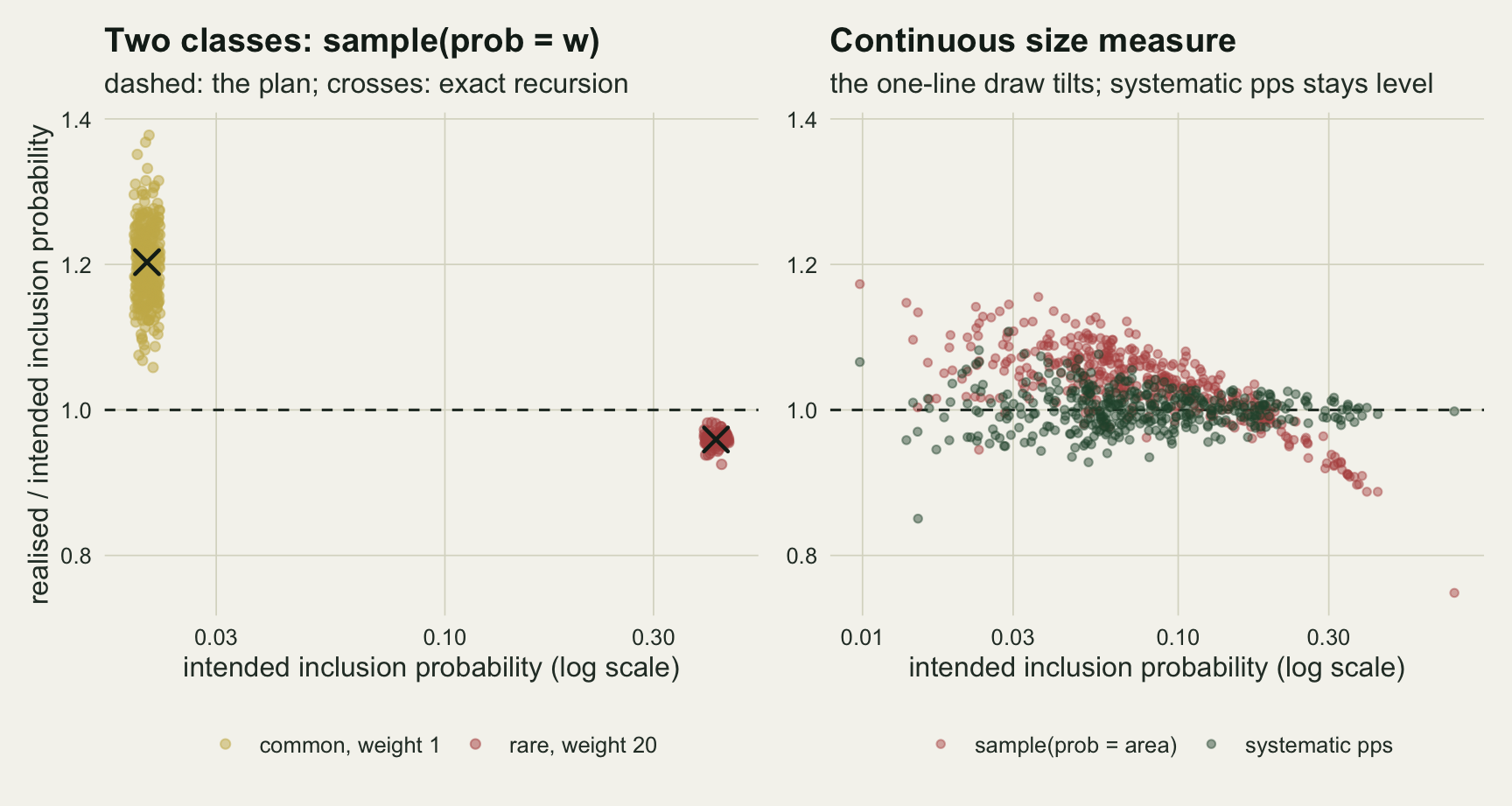
The Horvitz-Thompson mean inherits the gap
The Horvitz-Thompson mean divides each sampled value by its inclusion probability, sums, and divides by the number of sites in the frame. It is unbiased when the probabilities it divides by are the probabilities the draw actually used. Here the analyst divides by the intended ones. The comparison below runs 5000 fresh draws per frame and computes the estimator twice from each draw: once with the intended probabilities, as the analyst would, and once with the realised probabilities estimated by simulation in the previous section.
n_rep <- 5000
rel_bias <- function(est, truth) 100 * (mean(est) - truth) / truth
rel_se   <- function(est, truth) 100 * sd(est) / sqrt(length(est)) / truth
rel_sd   <- function(est, truth) 100 * sd(est) / truth

set.seed(52)
ht_succ <- lapply(seq_len(n_frame), function(i) {
  fr <- frames[[i]]
  est_int <- est_real <- numeric(n_rep)
  for (r_i in seq_len(n_rep)) {
    picked <- sample.int(n_site, n_draw, prob = fr$wt)
    est_int[r_i]  <- sum(fr$rich[picked] / fr$pip[picked]) / n_site
    est_real[r_i] <- sum(fr$rich[picked] / pi_mc[[i]][picked]) / n_site
  }
  list(int = est_int, real = est_real)
})
true_mean <- vapply(frames, function(fr) mean(fr$rich), 0)
bias_int  <- vapply(seq_len(n_frame), function(i) rel_bias(ht_succ[[i]]$int, true_mean[i]), 0)
bias_real <- vapply(seq_len(n_frame), function(i) rel_bias(ht_succ[[i]]$real, true_mean[i]), 0)
se_int    <- vapply(seq_len(n_frame), function(i) rel_se(ht_succ[[i]]$int, true_mean[i]), 0)
se_real   <- vapply(seq_len(n_frame), function(i) rel_se(ht_succ[[i]]$real, true_mean[i]), 0)
sd_int    <- vapply(seq_len(n_frame), function(i) rel_sd(ht_succ[[i]]$int, true_mean[i]), 0)

## the same bias from the exact class probabilities, no estimator simulation
bias_exact <- vapply(frames, function(fr) {
  ratio_site <- ifelse(fr$is_rare, ratio_rare_exact, ratio_comm_exact)
  100 * sum(fr$rich * (ratio_site - 1)) / sum(fr$rich)
}, 0)

## why the sign is positive: the fixed sample size makes the two classes'
## changes in expected site count cancel, but a site enters the estimate
## as richness / intended probability, which differs between the classes
site_shift   <- n_rare * (pip_rare - pi_rare_exact)
per_site_comm <- mean_comm / pip_comm
per_site_rare <- mean_rare / pip_rare
With the intended probabilities the Horvitz-Thompson mean is biased upward by a median 5.60 per cent across the six frames (range 5.14 to 5.74), with a Monte Carlo standard error of about 0.18 per cent on each frame. With the realised probabilities the median is +0.08 per cent (range -0.20 to +0.33). The exact recursion predicts a bias of 5.40 to 5.90 per cent on the same frames without simulating a single estimate, because the expected value of the estimator is the sum of each site’s value times its realised-over-intended ratio.
The sign should surprise nobody who has followed the previous section, and its source can be stated exactly. Common sites are selected 1.203 times as often as planned, and each still carries the large weight of a rarely sampled site, so their contribution to the estimate is inflated by that factor; rare sites are deflated by 0.959. The fixed sample size forces the two shifts to cancel in sites: the rare class loses 1.35 expected sites and the common class gains exactly as many. In the estimator, though, each site counts as its richness divided by its intended probability, 240 for a common site of average richness against 72 for a rare one, so the extra common sites add more than the missing rare sites remove. The size of the bias therefore depends on how richness per site compares with the weight in each class, which the designer of this example chose; the section after next takes that dependence apart.
Simulating the realised probabilities and dividing by them does remove the bias. The survey-design post runs its check before the field season, when a failure can still change the design; after the fact, dividing by simulated probabilities is the only repair left, and a poor one. It needs a simulation of every design before every analysis, the probabilities it produces carry Monte Carlo error into every weight, and the draw is still not the design anyone wrote in a protocol. The better repair is a draw that delivers the written design.
Two samplers that hit the plan
Two unequal-probability designs deliver the intended first-order probabilities exactly and take a few lines of base R.
Systematic sampling with probability proportional to size (Madow 1949, there in a given order; the random-order version and its variance are analysed by Hartley and Rao 1962) puts the sites in a random order, lays their intended probabilities end to end along a line of length 40, takes one uniform random start in the first unit interval, and selects the site under that start and under each of the 39 points spaced one apart after it. Each site is covered by a stretch of the line exactly as long as its probability, so it is selected with exactly that probability, and the sample size is always 40. This is also the draw inside the GRTS function of the spatial-sampling posts, which follows Stevens and Olsen: there the order is the spatial address instead of a random permutation, which is why check one passes in the survey-design post and why the Horvitz-Thompson conclusion in the unequal-probability post holds for its draw.
Poisson sampling flips an independent coin for every site with that site’s intended probability. It is exact by construction and trivial to code; the price is that the sample size is random.
poisson_draw <- function(pip) which(runif(length(pip)) < pip)

set.seed(53)
ht_other <- lapply(seq_len(n_frame), function(i) {
  fr <- frames[[i]]
  est_madow <- est_pois <- est_hajek <- numeric(n_rep)
  size_pois <- integer(n_rep)
  for (r_i in seq_len(n_rep)) {
    picked <- madow_draw(fr$pip, n_draw)
    est_madow[r_i] <- sum(fr$rich[picked] / fr$pip[picked]) / n_site
    picked <- poisson_draw(fr$pip)
    est_pois[r_i]  <- sum(fr$rich[picked] / fr$pip[picked]) / n_site
    est_hajek[r_i] <- sum(fr$rich[picked] / fr$pip[picked]) / sum(1 / fr$pip[picked])
    size_pois[r_i] <- length(picked)
  }
  list(madow = est_madow, pois = est_pois, hajek = est_hajek, size = size_pois)
})
bias_madow <- vapply(seq_len(n_frame), function(i) rel_bias(ht_other[[i]]$madow, true_mean[i]), 0)
bias_pois  <- vapply(seq_len(n_frame), function(i) rel_bias(ht_other[[i]]$pois, true_mean[i]), 0)
bias_hajek <- vapply(seq_len(n_frame), function(i) rel_bias(ht_other[[i]]$hajek, true_mean[i]), 0)
se_madow   <- vapply(seq_len(n_frame), function(i) rel_se(ht_other[[i]]$madow, true_mean[i]), 0)
se_pois    <- vapply(seq_len(n_frame), function(i) rel_se(ht_other[[i]]$pois, true_mean[i]), 0)
sd_madow   <- vapply(seq_len(n_frame), function(i) rel_sd(ht_other[[i]]$madow, true_mean[i]), 0)
sd_pois    <- vapply(seq_len(n_frame), function(i) rel_sd(ht_other[[i]]$pois, true_mean[i]), 0)
sd_hajek   <- vapply(seq_len(n_frame), function(i) rel_sd(ht_other[[i]]$hajek, true_mean[i]), 0)
size_sd    <- median(vapply(ht_other, function(h) sd(h$size), 0))
size_range <- range(unlist(lapply(ht_other, function(h) range(h$size))))
max_z_exact <- max(abs(c(bias_madow / se_madow, bias_pois / se_pois)))
n_comm_expected <- (n_site - n_rare) * pip_comm
On the same six frames and with the same intended probabilities, the Horvitz-Thompson mean has a median bias of +0.03 per cent under systematic pps (range -0.15 to +0.07) and -0.002 per cent under Poisson sampling (range -0.45 to +0.37). The Monte Carlo standard errors are about 0.18 and 0.26 per cent, and no frame is further from zero than 1.8 of its own standard errors, which is what an unbiased estimator produces over 5000 draws. Nothing about the weights or the estimator changed; only the line that draws the sample.
The two samplers are not equally good, and the difference is precision. The standard deviation of a single survey’s estimate, as a percentage of the true mean, is a median 12.6 for the one-line draw, 12.9 for systematic pps and 18.5 for Poisson sampling. Systematic pps in a random order is slightly less precise than the draw it replaces, but not by much. Poisson sampling pays for its simplicity with a sample size that varied from 20 to 61 sites across draws (standard deviation 5.1), and with the extra variance that brings. The usual remedy for a random sample size, dividing by the estimated frame size instead of the known one (the Hajek form), makes things worse on this frame: its median bias is +5.65 per cent and its standard deviation 23.0, because only 6.67 common sites are expected in each sample and the estimated frame size swings with their number.
fr_one <- frames[[1]]
set.seed(54)
v_madow <- est_m <- v_pois <- est_p <- numeric(n_rep)
for (r_i in seq_len(n_rep)) {
  picked <- madow_draw(fr_one$pip, n_draw)
  z_val  <- n_draw * fr_one$rich[picked] / fr_one$pip[picked]
  est_m[r_i]   <- mean(z_val) / n_site
  v_madow[r_i] <- var(z_val) / n_draw / n_site^2
  picked <- poisson_draw(fr_one$pip)
  est_p[r_i]  <- sum(fr_one$rich[picked] / fr_one$pip[picked]) / n_site
  v_pois[r_i] <- sum((1 - fr_one$pip[picked]) * fr_one$rich[picked]^2 /
                       fr_one$pip[picked]^2) / n_site^2
}
ratio_v_madow <- mean(v_madow) / var(est_m)
ratio_v_pois  <- mean(v_pois) / var(est_p)
cover_madow <- mean(abs(est_m - true_mean[1]) <= qnorm(0.975) * sqrt(v_madow))
cover_pois  <- mean(abs(est_p - true_mean[1]) <= qnorm(0.975) * sqrt(v_pois))
cover_se    <- sqrt(0.95 * 0.05 / n_rep)
cor_pois    <- cor(est_p, sqrt(v_pois))
miss_high   <- mean(est_p - true_mean[1] > qnorm(0.975) * sqrt(v_pois))
miss_low    <- mean(true_mean[1] - est_p > qnorm(0.975) * sqrt(v_pois))

## exact variances of two reference designs on the same frame, for comparison
## with the simulated variance of systematic pps in a random order
z_pop <- fr_one$rich / fr_one$pip
p_wr  <- fr_one$pip / n_draw
v_wr_exact <- sum(p_wr * (fr_one$rich / p_wr - sum(fr_one$rich))^2) / n_draw / n_site^2
c_pop <- n_site / (n_site - 1) * fr_one$pip * (1 - fr_one$pip)
v_hd_pop <- sum(c_pop * (z_pop - sum(c_pop * z_pop) / sum(c_pop))^2) / n_site^2
ratio_madow_wr <- var(est_m) / v_wr_exact
ratio_madow_hd <- var(est_m) / v_hd_pop
The recommendation depends on what else the survey needs. Systematic pps is fixed in size, but its joint inclusion probabilities have no convenient form, so its variance has to be approximated. The simplest approximation treats the sample as if it had been drawn with replacement, and on this frame that flatters the design: the variance of the systematic estimates across draws on the first frame is 1.14 times the exact variance of with-replacement pps, so the random-order systematic draw is less precise than a with-replacement draw would be. Built from one sample at a time, the approximation averaged 0.88 of the variance across draws, and nominal 95 per cent intervals built on it covered the true mean in 0.879 of 5000 draws (Monte Carlo standard error 0.003). A more refined approximation does not help here. Hajek’s approximation for fixed-size designs of high entropy, one of those in Tille’s book, is smaller still: the systematic variance is 1.26 times it, so intervals built on it would miss more often. Poisson sampling has an exact unbiased variance estimator, because its sites are selected independently; its average is 1.06 of the variance across draws, and the same intervals covered 0.927, short of 0.95. The misses are lopsided: 0.068 of the intervals fell wholly below the truth and 0.005 wholly above it. A sample that happens to hold few of the heavily weighted common sites gives a low estimate and a low variance estimate together (their correlation across draws is 0.87), so the low estimates come with intervals that are too narrow.
## conditional Poisson (maximum-entropy) sampling, exact for two classes:
## the number of rare sites k has probability proportional to
## choose(80, k) * choose(320, 40 - k) * theta^k, and theta is set so
## that the expected number of rare sites is the planned 80 * pip_rare
k_all   <- 0:n_draw
lw_base <- lchoose(n_rare, k_all) + lchoose(n_site - n_rare, n_draw - k_all)
k_dist  <- function(log_theta) {
  lw <- lw_base + k_all * log_theta
  exp(lw - max(lw)) / sum(exp(lw - max(lw)))
}
log_theta <- uniroot(function(lt) sum(k_all * k_dist(lt)) - n_rare * pip_rare,
                     c(-10, 20), tol = 1e-12)$root
prob_k <- k_dist(log_theta)
maxent_draw <- function(fr) {
  k_rare <- sample(k_all, 1, prob = prob_k)
  c(sample(which(fr$is_rare), k_rare), sample(which(!fr$is_rare), n_draw - k_rare))
}

set.seed(58)
est_c <- v_c <- numeric(n_rep)
rare_c <- integer(n_rep)
for (r_i in seq_len(n_rep)) {
  picked <- maxent_draw(fr_one)
  z_val  <- fr_one$rich[picked] / fr_one$pip[picked]
  c_k    <- 1 - fr_one$pip[picked]
  est_c[r_i] <- sum(z_val) / n_site
  v_c[r_i]   <- n_draw / (n_draw - 1) *
    sum(c_k * (z_val - sum(c_k * z_val) / sum(c_k))^2) / n_site^2
  rare_c[r_i] <- sum(fr_one$is_rare[picked])
}
ratio_rare_c <- mean(rare_c) / n_rare / pip_rare
bias_c  <- rel_bias(est_c, true_mean[1])
se_c    <- rel_se(est_c, true_mean[1])
sd_c    <- rel_sd(est_c, true_mean[1])
ratio_v_c <- mean(v_c) / var(est_c)
cover_c   <- mean(abs(est_c - true_mean[1]) <= qnorm(0.975) * sqrt(v_c))
miss_low_c  <- mean(true_mean[1] - est_c > qnorm(0.975) * sqrt(v_c))
miss_high_c <- mean(est_c - true_mean[1] > qnorm(0.975) * sqrt(v_c))
## the same intervals with the variance across draws in place of each
## sample's own estimate, and how that estimate moves with the estimate
cover_c_known <- mean(abs(est_c - true_mean[1]) <= qnorm(0.975) * sd(est_c))
cor_c <- cor(est_c, sqrt(v_c))
A fixed-size design whose variance Hajek’s approximation does describe is conditional Poisson, or maximum-entropy, sampling: Poisson samples conditioned on having exactly the planned size, with working probabilities adjusted until the first-order probabilities come out as intended. With two classes it can be drawn exactly in a few lines, because within a class the sites are exchangeable and only the number of rare sites in the sample needs a distribution. On the first frame its rare-class ratio is 0.9997 of the plan and the Horvitz-Thompson mean has a bias of +0.08 per cent (Monte Carlo standard error 0.16). The standard deviation of a single survey’s estimate is 11.2 per cent, against 12.4 for the one-line draw and 12.5 for systematic pps on the same frame, and Hajek’s variance approximation, computed from each sample with an n/(n-1) correction, averages 1.03 of the variance across draws.
The variance approximation is right on average, and the intervals still cover only 0.901, with the same lopsided misses as under Poisson sampling (0.093 wholly below the truth, 0.006 wholly above). The cause is the one described there. The estimate itself is not the problem: with the variance across draws in place of each sample’s own estimate, the same intervals cover 0.950. But each sample’s variance estimate rests on the same handful of heavily weighted common sites as its mean, so the two rise and fall together (correlation 0.86), and a sample with few common sites gets a low estimate and an interval too narrow to reach the truth. A variance formula that is right on average does not remove that. For a programme with a fixed field budget that reports a landscape mean with an interval, a maximum-entropy draw is the better choice of the three fixed-size draws here: exact first-order probabilities, the smallest standard deviation on this frame, and a variance approximation that fits. For a general size measure it is UPmaxentropy() in the CRAN package sampling that the help page points to, which also has Sampford’s method (UPsampford()), another fixed-size design with computable joint probabilities; neither function was run here. Systematic pps is the simpler choice when only the point estimate matters, and Poisson sampling suits a programme that can live with a variable number of visits, at the cost of a wider interval. Whichever is used, the coverage on a frame like this one should be checked by simulating the design, because the nominal level is not what the reader gets.
cal_gap <- function(wt_try) {
  succ_prob_rare(n_draw, n_rare, n_site - n_rare, wt_try, wt_comm) - pip_rare
}
wt_cal <- uniroot(cal_gap, c(wt_rare, 10 * wt_rare), tol = 1e-10)$root
wt_cal_check <- succ_prob_rare(n_draw, n_rare, n_site - n_rare, wt_cal, wt_comm) / pip_rare
set.seed(55)
wt_cal_vec <- ifelse(fr_one$is_rare, wt_cal, wt_comm)
est_cal <- replicate(n_rep, {
  picked <- sample.int(n_site, n_draw, prob = wt_cal_vec)
  sum(fr_one$rich[picked] / fr_one$pip[picked]) / n_site
})
bias_cal <- rel_bias(est_cal, true_mean[1])
se_cal   <- rel_se(est_cal, true_mean[1])
There is a third way out that keeps sample(): change the prob argument until the successive draw lands on the intended probabilities. With two classes the recursion solves it exactly. A rare-class weight of 25.45 instead of 20 brings the realised rare-class probability to 1.0000 of the plan, and the Horvitz-Thompson mean with the intended probabilities then has a bias of +0.07 per cent on the first frame (Monte Carlo standard error 0.16). This is a patch for the two-class case rather than a method: with a continuous size measure the calibration has to be done by simulation, the weights change with n, and a protocol that says “weight 20” while the code says something else is a protocol no one can reproduce from the text.
bias_df <- data.frame(
  frame = rep(seq_len(n_frame), 4),
  arm = rep(c("sample(), intended pi", "sample(), simulated realised pi",
              "systematic pps, intended pi", "Poisson, intended pi"), each = n_frame),
  bias = c(bias_int, bias_real, bias_madow, bias_pois),
  se = c(se_int, se_real, se_madow, se_pois))
arm_levels <- unique(bias_df$arm)
bias_df$arm_pos <- match(bias_df$arm, rev(arm_levels)) + (bias_df$frame - 3.5) * 0.09

ggplot(bias_df, aes(bias, arm_pos, colour = arm)) +
  geom_vline(xintercept = 0, linetype = "dashed", colour = te_body) +
  geom_errorbar(aes(xmin = bias - 2 * se, xmax = bias + 2 * se),
                orientation = "y", width = 0, linewidth = 0.5) +
  geom_point(size = 2.2) +
  scale_y_continuous(breaks = seq_along(arm_levels), labels = rev(arm_levels)) +
  scale_colour_manual(values = c(te_rust, te_gold, te_forest, te_ink), guide = "none") +
  labs(x = "relative bias of the landscape mean (per cent)", y = NULL,
       title = "Change the draw, not the weights",
       subtitle = "one point per frame; dashed: unbiased") +
  theme_datasheet()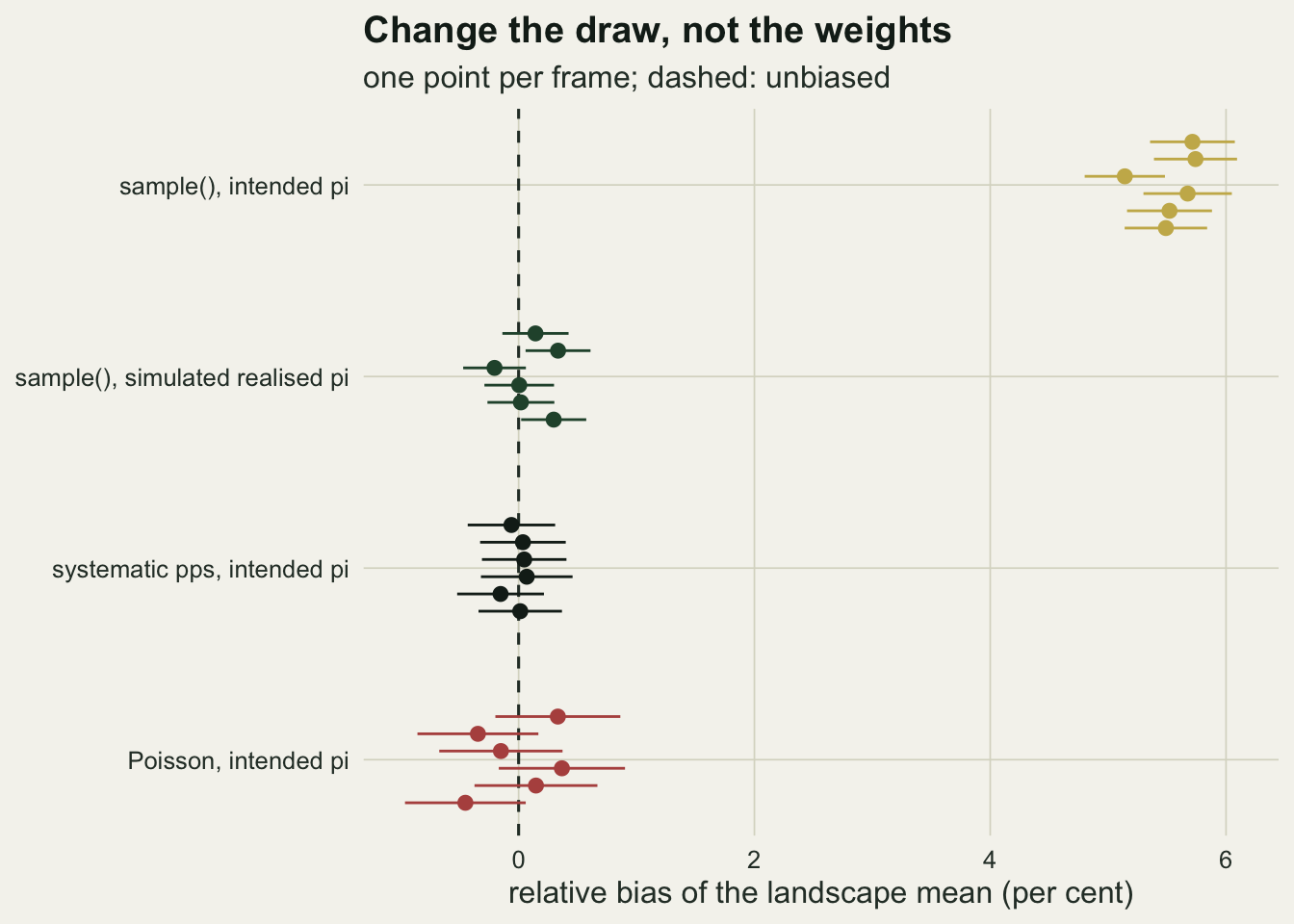
The bias grows as the weight says less
A survey statistician’s first question about a result like this is whether the 5.6 per cent is an artefact of the chosen richness contrast, and whether it shrinks when the weight is only loosely related to the variable of interest, which is the usual case. The exact recursion answers it without further simulation. Because a site’s expected contribution to the estimate is its value times its realised-over-intended ratio, and the two classes’ ratios are tied together by the fixed sample size, the bias is proportional to the rare-class mean minus 20 times the common-class mean. It is zero when richness is exactly proportional to the weight, which is the textbook pps situation of sampling proportional to a size that predicts the variable, and it grows as richness departs from proportionality in either direction.
ratio_grid <- exp(seq(log(1), log(40), length.out = 60))
bias_curve <- function(mean_ratio) {
  tot_rare <- n_rare * mean_ratio
  tot_comm <- (n_site - n_rare) * 1
  100 * (tot_rare * (ratio_rare_exact - 1) + tot_comm * (ratio_comm_exact - 1)) /
    (tot_rare + tot_comm)
}
curve_df <- data.frame(ratio = ratio_grid, bias = bias_curve(ratio_grid))
bias_at_equal <- bias_curve(1)
bias_at_design <- bias_curve(mean_rare / mean_comm)
bias_at_40 <- bias_curve(40)
bias_at_half <- bias_curve(0.5)

check_means <- c(5, 100)
set.seed(56)
check_df <- do.call(rbind, lapply(check_means, function(m_rare) {
  fr <- frames[[1]]
  rich_chk <- rpois(n_site, ifelse(fr$is_rare, m_rare, mean_comm))
  est_chk <- replicate(n_rep, {
    picked <- sample.int(n_site, n_draw, prob = fr$wt)
    sum(rich_chk[picked] / fr$pip[picked]) / n_site
  })
  data.frame(ratio = m_rare / mean_comm,
             bias = rel_bias(est_chk, mean(rich_chk)),
             se = rel_se(est_chk, mean(rich_chk)),
             pred = 100 * sum(rich_chk * (ifelse(fr$is_rare, ratio_rare_exact,
                                                  ratio_comm_exact) - 1)) / sum(rich_chk))
}))
When the two classes have the same mean richness, so that the weight tells the design nothing about richness at all, the bias is 15.4 per cent, nearly three times the 5.7 per cent at the chosen design’s class means. At a ratio of 20 it is zero, and when the rare class is richer than proportional it turns negative, reaching -1.8 per cent at a ratio of 40. Two direct simulations check the curve on the first frame with fresh richness values: with equal class means the simulated bias is 15.68 per cent against a prediction of 15.26, and at a ratio of 20 it is -0.09 against -0.07 (Monte Carlo standard errors 0.44 and 0.05).
So the usual case is the bad case. An ecologist oversamples a rare habitat for coverage, not because the habitat predicts the response in proportion to the weight, and the further the response is from that proportionality, the larger the bias. The equal-means end of the curve is also a check any reader can run on their own design with no response data at all: it is the relative bias of the Horvitz-Thompson estimate of the frame size, the sum of one over the intended probability across the sample, which should average to the number of sites.
sim_pts <- rbind(check_df[, c("ratio", "bias", "se")],
                 data.frame(ratio = vapply(frames, function(fr)
                              mean(fr$rich[fr$is_rare]) / mean(fr$rich[!fr$is_rare]), 0),
                            bias = bias_int, se = se_int))
ggplot(curve_df, aes(ratio, bias)) +
  geom_hline(yintercept = 0, colour = te_body, linewidth = 0.4) +
  geom_vline(xintercept = wt_rare / wt_comm, linetype = "dashed", colour = te_body) +
  geom_line(colour = te_forest, linewidth = 1) +
  geom_errorbar(data = sim_pts, aes(ymin = bias - 2 * se, ymax = bias + 2 * se),
                width = 0, colour = te_rust, linewidth = 0.5) +
  geom_point(data = sim_pts, colour = te_rust, size = 2.2) +
  scale_x_log10(breaks = c(1, 2, 5, 10, 20, 40)) +
  labs(x = "rare-class mean richness / common-class mean richness",
       y = "relative bias (per cent)",
       title = "Proportional to the weight is the only safe case",
       subtitle = "curve: exact; points: simulated; dashed: weight ratio 20") +
  theme_datasheet()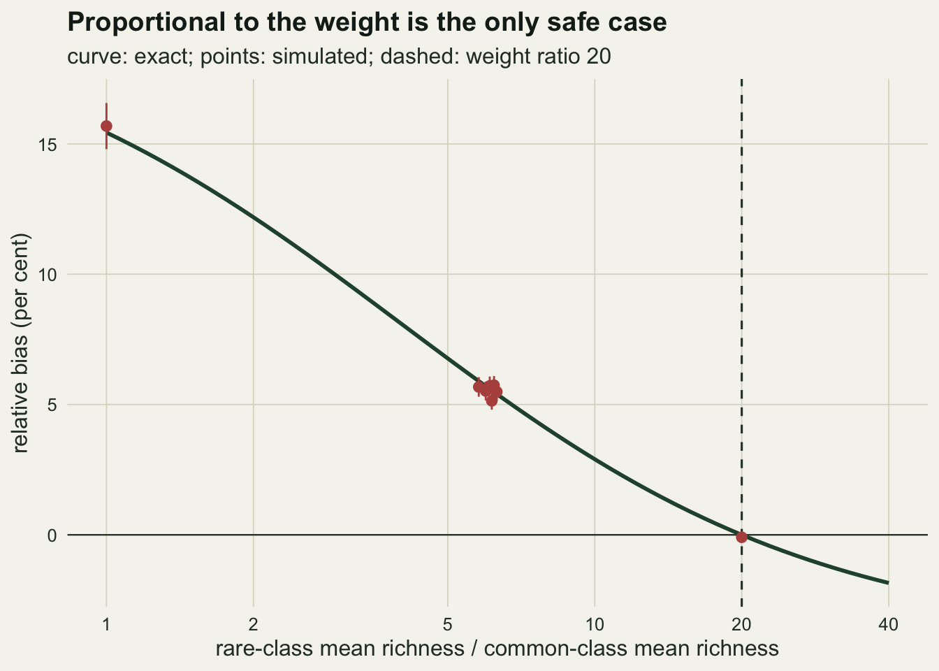
Larger samples, larger distortion
The other review question is where the effect stops mattering. The distortion has to vanish for a sample of one, where the first pick uses the weights exactly, and it grows as the sample takes a larger share of the rare class out of the pool. Against it stands the sampling error of a single survey, which shrinks as the sample grows. The sweep below holds the frame and the weights fixed and varies the sample size, computing the probability distortion and the bias exactly from the recursion and the standard deviation of the estimate from 4000 draws on the first frame.
n_grid <- c(10, 20, 40, 60, 80)
n_sweep <- 4000
set.seed(57)
frac_tab <- do.call(rbind, lapply(n_grid, function(n_pick) {
  pip_n  <- n_pick * fr_one$wt / sum(fr_one$wt)
  pr_rare <- succ_prob_rare(n_pick, n_rare, n_site - n_rare, wt_rare, wt_comm)
  pr_comm <- (n_pick - n_rare * pr_rare) / (n_site - n_rare)
  r_rare <- pr_rare / pip_n[fr_one$is_rare][1]
  r_comm <- pr_comm / pip_n[!fr_one$is_rare][1]
  bias_n <- 100 * sum(fr_one$rich * (ifelse(fr_one$is_rare, r_rare, r_comm) - 1)) /
    sum(fr_one$rich)
  est_n <- replicate(n_sweep, {
    picked <- sample.int(n_site, n_pick, prob = fr_one$wt)
    sum(fr_one$rich[picked] / pip_n[picked]) / n_site
  })
  data.frame(n_pick = n_pick, frac = n_pick / n_site, max_pip = max(pip_n),
             r_rare = r_rare, bias = bias_n, sd_est = rel_sd(est_n, true_mean[1]))
}))
frac_tab$bias_over_sd <- frac_tab$bias / frac_tab$sd_est
n_cap <- 0.25 * n_site
pip_cap <- n_cap * wt_rare / sum(fr_one$wt)
row_40 <- which(frac_tab$n_pick == n_draw)
At a sampling fraction of 0.025 the rare class comes in at 0.992 of its intended rate and the bias is 1.04 per cent, 0.04 of a single survey’s standard deviation. At the design’s 0.10 the bias is 0.45 of a standard deviation, and at 0.20 the rare-class ratio has fallen to 0.888, the bias is 14.8 per cent, and it is 1.71 of a standard deviation. The sweep stops at a fraction of 0.2 on purpose: at 0.25 the rare-class probability would be 1.042, above one, and the design would need capping, which is a different failure owned by the survey-design post.
For a single small survey, then, the bias hides inside the sampling noise, and the reader who wants to argue that it does not matter can find a fraction where that is true. Two things weigh against that argument. A bias does not average away: a programme that pools years, compares regions or feeds the estimate into a trend model accumulates it while the noise shrinks. And the trade-off the question implies, bias against the precision gained by oversampling, does not exist, because an exact sampler removes the bias at little or no cost in precision: systematic pps gives up a little on these frames, and the maximum-entropy draw gains some on the first. There is no fraction at which the one-line draw is the better choice, only fractions at which it is not yet visibly worse.
p_ratio <- ggplot(frac_tab, aes(frac, r_rare)) +
  geom_hline(yintercept = 1, linetype = "dashed", colour = te_body) +
  geom_line(colour = te_rust, linewidth = 0.9) +
  geom_point(colour = te_rust, size = 2.4) +
  labs(x = "sampling fraction n / N", y = "realised / intended, rare site",
       title = "The rare class slips",
       subtitle = "dashed: the plan") +
  theme_datasheet()
p_share <- ggplot(frac_tab, aes(frac, bias_over_sd)) +
  geom_hline(yintercept = 0, colour = te_body, linewidth = 0.4) +
  geom_line(colour = te_forest, linewidth = 0.9) +
  geom_point(colour = te_forest, size = 2.4) +
  labs(x = "sampling fraction n / N", y = "bias / standard deviation",
       title = "and the bias outgrows the noise",
       subtitle = "one survey's standard deviation as the yardstick") +
  theme_datasheet()
p_ratio + p_share + plot_annotation(theme = theme_datasheet())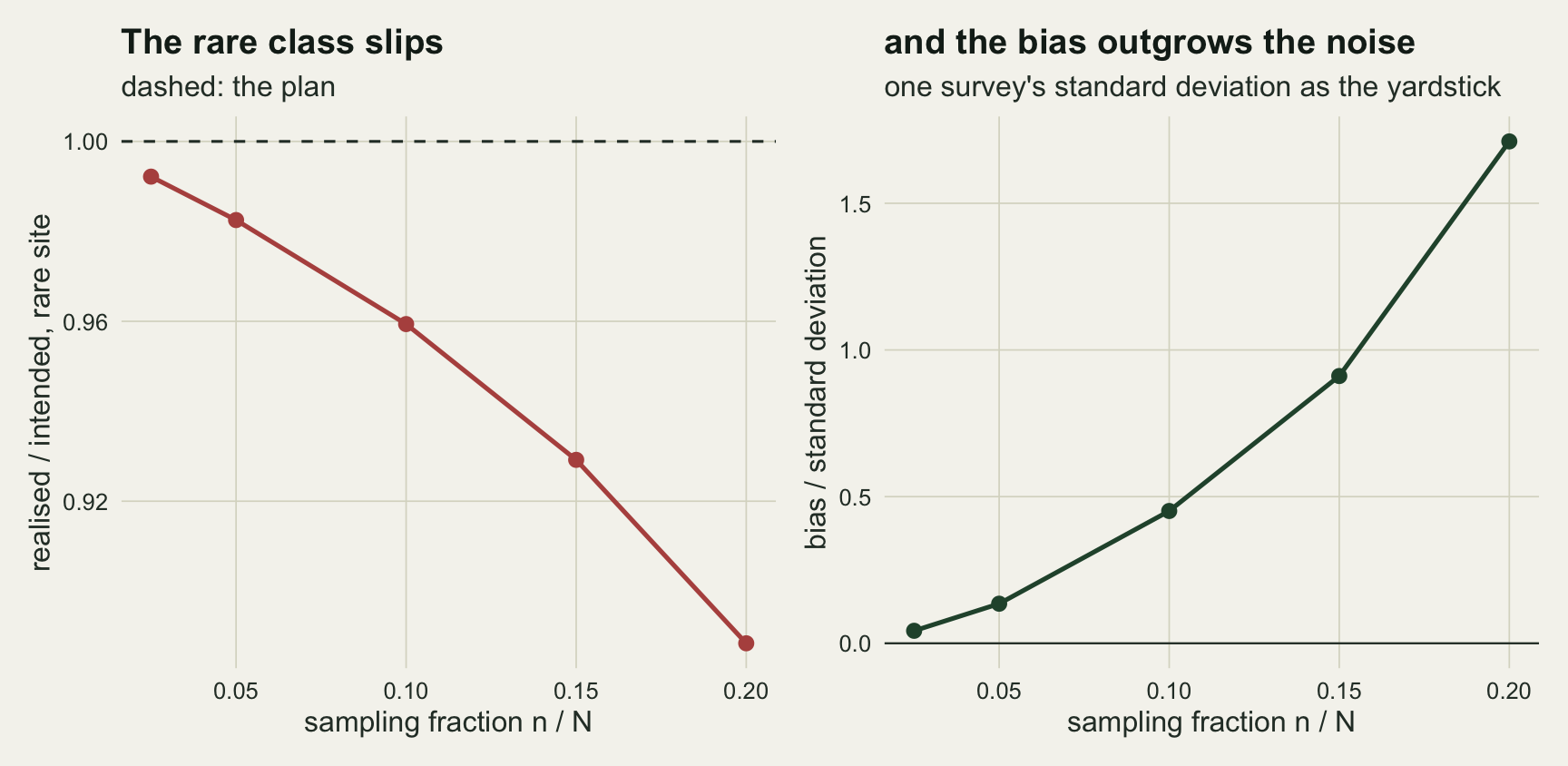
What to report
Name the sampler, not just the probabilities. A methods section that says “sites were selected with probability proportional to weight” describes a design; sample(prob = w) without replacement does not implement it, and the reader cannot tell which happened unless the draw is named. “Systematic pps with a random order (Madow 1949; Hartley and Rao 1962)”, “conditional Poisson (maximum-entropy) sampling”, “Poisson sampling” and “GRTS” each name a draw whose first-order probabilities are the ones written down.
If an existing survey was drawn with the one-liner, the damage is repairable because the design is known. Compute the realised inclusion probabilities, exactly by the recursion when the weights fall in a few classes or by simulation of the actual draw otherwise, and use those in the estimator. Report that this was done, and report the realised rare-class ratio, 0.959 in the example here, so a reader can judge the size of the correction.
Report the sampling fraction and the weight ratio alongside the estimate. The distortion grows with the sampling fraction and disappears when the weights are equal, and the bias it produces depends on how far the response is from proportional to the weight, large when the weight has nothing to do with the response, and larger still when the oversampled class is the poorer one (17.6 per cent in the example if rare sites held half the richness of common ones). A check any reader can run is the Horvitz-Thompson estimate of the frame size itself: under the one-line draw in the example its relative bias is the 15.4 per cent of the equal-means case, and under an exact sampler it is zero.
If systematic pps is used, report the variance approximation and, if possible, check its coverage by simulation of the design as done above; the with-replacement approximation covered 0.879 rather than 0.95 on this frame, and even the maximum-entropy draw, with a variance approximation that fits, covered 0.901.
Honest limits
The frame is a two-class caricature with one continuous variant. Real designs mix strata, several weight levels and a size measure, and the distortion then differs unit by unit; the recursion used here covers only the class structure, and anything richer needs the simulation.
The exactness claims for systematic pps and Poisson sampling are about first-order inclusion probabilities. Systematic pps in a random order has joint probabilities with no simple closed form, so its variance must be approximated; the with-replacement approximation covered below its nominal level, and Hajek’s was compared only through its exact population value, not as an interval. The maximum-entropy draw was implemented only for two classes, where it can be drawn exactly, and on the first frame only; Sampford’s method was not implemented, and neither was the sampling package, which is not among the packages this post uses. The under-coverage that survives a variance approximation that is right on average comes from the estimate and its variance estimate resting on the same handful of heavily weighted common sites in each sample; how it changes with the weight ratio was not measured.
The richness model is Poisson with two class means and no spatial structure. Nothing in the bias arithmetic depends on the Poisson form, but the Monte Carlo standard errors and the coverage figures do, and a heavier-tailed response would likely lower the coverage of every interval above.
The calibrated-weight patch was solved exactly for two classes and checked on one frame. It is shown to make the point that the fault lies in the mapping from weights to probabilities, not as a recommendation.
Finally, the neighbour posts are not wrong. The Horvitz-Thompson conclusion in the unequal-probability post and the passing check in the survey-design post are both true of the draw those posts use, which is a systematic pps draw along a spatial order. What fails is carrying their conclusion over to a different line of code.
References
Horvitz DG, Thompson DJ 1952 Journal of the American Statistical Association 47(260):663-685 (10.1080/01621459.1952.10483446)
Madow WG 1949 The Annals of Mathematical Statistics 20(3):333-354 (10.1214/aoms/1177729988)
Hartley HO, Rao JNK 1962 The Annals of Mathematical Statistics 33(2):350-374 (10.1214/aoms/1177704564)
Brewer KRW, Hanif M 1983 Sampling with Unequal Probabilities, Lecture Notes in Statistics, Springer (10.1007/978-1-4684-9407-5)
Tille Y 2006 Sampling Algorithms, Springer Series in Statistics (10.1007/0-387-34240-0)
Stevens DL, Olsen AR 2004 Journal of the American Statistical Association 99(465):262-278 (10.1198/016214504000000250)