library(ggplot2)

te_paper  <- "#f5f4ee"
te_ink    <- "#16241d"
te_body   <- "#2c3a31"
te_forest <- "#275139"
te_rust   <- "#b5534e"
te_gold   <- "#c9b458"
te_line   <- "#dad9ca"

theme_datasheet <- function() {
  theme_minimal(base_size = 12) +
    theme(plot.background  = element_rect(fill = te_paper, colour = NA),
          panel.background = element_rect(fill = te_paper, colour = NA),
          panel.grid.major = element_line(colour = te_line, linewidth = 0.3),
          panel.grid.minor = element_blank(),
          text             = element_text(colour = te_body),
          plot.title       = element_text(colour = te_ink, face = "bold"),
          plot.subtitle    = element_text(colour = te_body),
          axis.text        = element_text(colour = te_body))
}

fmt_e <- function(x) formatC(x, format = "e", digits = 2)When integrate() in R returns zero and says OK
R
numerical methods
measurement error
likelihood
reproducibility
ecology tutorial
R’s integrate() returns zero and says OK for a density far from the origin. How it breaks a measurement-error likelihood, and which change of variable fixes it.
A fisheries student is fitting length at maturity. Each fish was measured with callipers to within a few millimetres, the lengths sit around 420 mm, and the model is a logistic regression of maturity on true length, not on the recorded one, because the student has read that measurement error in a predictor drags a slope towards zero. The honest likelihood for one fish integrates over the length it might really have had, and the student writes that integral the way the help page writes it: integrate(f, -Inf, Inf). The fit runs, optim() reports convergence code 0, and the slope comes out with a sign nobody expected. Nothing printed a warning, and integrate() reported no trouble with any of the integrals behind that fit.
The mechanism is not new and this post claims no discovery. R’s integrate() is built on the QUADPACK routines of Piessens and colleagues, and for an infinite range it uses the dqagi transformation, which maps the whole real line onto a finite interval and then applies an adaptive Gauss-Kronrod rule there. The rule looks first where the transformed variable puts its points, and those points crowd around the origin of the original scale. A density that is narrow and sits far from zero can fall between them. The help page says as much in its Note, in general terms. What is measured here is how often that happens on the (mean, width) pairs an ecologist actually meets, what it does to a real likelihood fit, and which repair survives.
The tree already has 33 posts that call integrate(). Every one of them uses it, none shows it failing, and the calls with an infinite limit are all on integrands that are standardised, have their mass at zero, or are wide enough near the origin for the first probes to land on them: the half-normal detection function in call rates and density from acoustic surveys, the expected maximum of standard normals in the sap flow baseline post. A chi-square density with 76 degrees of freedom in home vs away and local vs foreign is the furthest out, and it integrates correctly. The site is safe by accident rather than by argument, and this post is the argument.
The nearest posts on the site are about computation choices too, and the difference matters. Eviction and mesh size in an IPM shows a midpoint rule under-resolving a narrow kernel, but the mesh is a number the analyst typed and the loss shows up in the kernel for anyone who plots it. Harmonics or cyclic splines for a narrow seasonal peak turns on REML against UBRE as a smoothing criterion, synthetic likelihood for noisy population dynamics on how many simulations to spend per evaluation, and fat tails and accelerating spread on grid width, zero padding and a declared floor. All of those are choices the analyst declared and can see in their own code; this one is an undeclared default inside a base R function, the analyst declared nothing, and the loss is printed as “OK”. Coordinate error and habitat assignment warns that “a quadrature rule built for smooth integrands has no error bound” on a discontinuous integrand over a finite region, which is the opposite problem: here the integrand is as smooth as a function can be. Parameter scale decides what optim() finds is the closest case of all, an optimiser misled by the scale of its parameters, and it is not what happens here: both routes below move the same intercept and slope, on the same scale, from the same start, and what differs is the objective itself, which the diagnostic section recomputes.
The Laplace approximation in R checks a finite-difference Hessian against the analytic one, finds them in agreement, and concludes that the numerical route is fine for a model whose derivatives you cannot face writing out. The habit that post teaches, checking the numerical answer against an exact one, is the habit that catches what follows. Measurement error and regression dilution and correcting measurement error with SIMEX are about what error in a predictor does to a slope and how to undo it. Those posts own the estimand this fit is trying to recover; this one is about the computation of that fit, and it is not a new correction.
Where integrate() looks
The quickest way to see the problem is to ask integrate() where it evaluated the function. The wrapper below records every point it was handed, for three normal densities: the standard normal from the help page, a density with mean 20 and standard deviation 1, and one with mean 420 and standard deviation 15, which is the true length distribution of the fish above.
probe_call <- function(mu, s) {
  seen <- numeric(0)
  res  <- integrate(function(x) {
    seen <<- c(seen, x)
    dnorm(x, mu, s)
  }, -Inf, Inf, stop.on.error = FALSE)
  list(res = res, pts = seen)
}

probe_mu <- c(0, 20, 420)
probe_sd <- c(1, 1, 15)
probe_out <- Map(probe_call, probe_mu, probe_sd)

probe_val  <- vapply(probe_out, function(p) p$res$value, 0)
probe_msg  <- vapply(probe_out, function(p) p$res$message, "")
probe_err  <- vapply(probe_out, function(p) p$res$abs.error, 0)
probe_n    <- vapply(probe_out, function(p) length(p$pts), 0)

pts_far    <- probe_out[[3]]$pts
n_near0    <- sum(abs(pts_far) < 10)
far_below  <- max(abs(pts_far)[abs(pts_far) < 420])
far_above  <- min(abs(pts_far)[abs(pts_far) > 420])
seen_max   <- max(dnorm(pts_far, 420, 15))
peak_far   <- dnorm(420, 420, 15)
seen_ratio <- seen_max / peak_far
For the standard normal the call returns 1.000000 with message "OK". For the mean of 20 it returns \(7.94 \times 10^{-7}\), and for the fish lengths it returns \(3.55 \times 10^{-67}\) with a reported absolute error of 0. All three messages read "OK" (all(probe_msg == "OK") returns TRUE). The calls were made with stop.on.error = FALSE. With the default, any failure the routine detects is raised as an error, so a value that comes back at all says OK; switching it off is what makes the message worth reading. The true answer is 1 in all three cases.
The fish-length call evaluated the density at 150 points. Of those, 124 lie within 10 mm of zero, a length no fish in the sample could have. The two probes nearest the mass sit at 233 mm and 467 mm, either side of a density whose mass lies within a few tens of millimetres of 420. The largest density value any probe saw was \(1.91 \times 10^{-4}\), which is 0.0072 of the peak.
Where those two probes came from explains the “OK”. QUADPACK integrates each piece of the transformed interval twice, with a 15-point Kronrod rule and with the 7-point Gauss rule whose points are a subset of it, and builds its error estimate from the gap between the two. The chunk below recomputes both rules by hand on the pieces the routine used, with the transformation x = (1 - t) / t that dqagi applies to both signs of x.
# nodes and weights of QUADPACK's 15-point Kronrod rule (half of the
# symmetric set) and of the 7-point Gauss rule embedded in it
xgk <- c(0.991455371120813, 0.949107912342759, 0.864864423359769,
         0.741531185599394, 0.586087235467691, 0.405845151377397,
         0.207784955007898, 0)
wgk <- c(0.022935322010529, 0.063092092629979, 0.104790010322250,
         0.140653259715525, 0.169004726639267, 0.190350578064785,
         0.204432940075298, 0.209482141084728)
wg  <- c(0.129484966168870, 0.279705391489277, 0.381830050505119,
         0.417959183673469)

gk_pair <- function(g, a, b) {
  cen <- (a + b) / 2
  hw  <- (b - a) / 2
  kron  <- hw * (sum(wgk[1:7] * (g(cen - hw * xgk[1:7]) + g(cen + hw * xgk[1:7]))) +
                   wgk[8] * g(cen))
  gauss <- hw * (sum(wg[1:3] * (g(cen - hw * xgk[c(2, 4, 6)]) +
                                  g(cen + hw * xgk[c(2, 4, 6)]))) + wg[4] * g(cen))
  c(kronrod = kron, gauss = gauss)
}
nodes_x <- function(a, b) {
  tt <- (a + b) / 2 + (b - a) / 2 * c(-xgk, rev(xgk[1:7]))
  (1 - tt) / tt
}

g_fish <- function(t) {
  x <- (1 - t) / t
  (dnorm(x, 420, 15) + dnorm(-x, 420, 15)) / t^2
}
first_half <- gk_pair(g_fish, 0, 0.5)
x_outer    <- max(nodes_x(0, 0.5))
kids_x     <- c(nodes_x(0, 0.25), nodes_x(0.25, 0.5))
kid_below  <- max(kids_x[kids_x < 420])
kid_above  <- min(kids_x[kids_x > 420])
final_sum  <- gk_pair(g_fish, 0, 0.25)["kronrod"] +
  gk_pair(g_fish, 0.25, 0.5)["kronrod"] + gk_pair(g_fish, 0.5, 1)["kronrod"]
hand_match <- abs(final_sum / probe_val[3] - 1)
The three pieces the routine finished on, recomputed this way, add up to the value integrate() returned to a relative difference of \(2.09 \times 10^{-12}\), so the hand rules are the ones it used. The probe at 467 mm is the outermost Kronrod point on the half of the transformed interval that covers |x| of 1 and more, and the embedded Gauss rule does not share it. On that half the Kronrod estimate was 0.240, about a quarter of the answer, and the Gauss estimate was \(3.79 \times 10^{-113}\). That disagreement is exactly what makes the routine split the piece, and neither new piece had a point between 156 mm and 935 mm. Both returned next to nothing, the error estimate for the total came out as 0, and the routine reported the result as a success.
probe_pm  <- function(x) {                 # "7.94" %*% 10^-7 for the strip labels
  s <- fmt_e(x)
  paste0('"', sub("e.*", "", s), '" %*% 10^', as.integer(sub(".*e", "", s)))
}
probe_lab <- sprintf('paste("mean %g, sd %g: returned ", %s)', probe_mu, probe_sd,
                     c(sprintf('"%.3f"', probe_val[1]), probe_pm(probe_val[2:3])))
probe_lab <- factor(probe_lab, levels = probe_lab)
x_curve   <- 10^seq(-3, 3.1, length.out = 3000)
curve_df  <- do.call(rbind, lapply(1:3, function(k) {
  dens <- dnorm(x_curve, probe_mu[k], probe_sd[k])
  data.frame(x = x_curve, y = dens / max(dens), call = probe_lab[k])
}))
tick_df <- do.call(rbind, lapply(1:3, function(k) {
  a <- abs(probe_out[[k]]$pts)
  a <- a[a > 1e-3]
  data.frame(x = a, call = probe_lab[k])
}))

ggplot() +
  geom_area(data = curve_df, aes(x, y), fill = te_forest, alpha = 0.25,
            colour = te_forest, linewidth = 0.6) +
  geom_segment(data = tick_df, aes(x = x, xend = x, y = -0.12, yend = -0.02),
               colour = te_rust, linewidth = 0.5) +
  facet_wrap(~ call, ncol = 1, labeller = label_parsed) +
  scale_x_log10(breaks = c(0.001, 0.01, 0.1, 1, 10, 100, 1000),
                labels = c("0.001", "0.01", "0.1", "1", "10", "100", "1000")) +
  labs(x = "absolute value of x (log scale)", y = "density / its peak",
       title = "The probes crowd near zero",
       subtitle = "red ticks: points where integrate() evaluated the function") +
  theme_datasheet() +
  theme(strip.text = element_text(colour = te_ink, hjust = 0))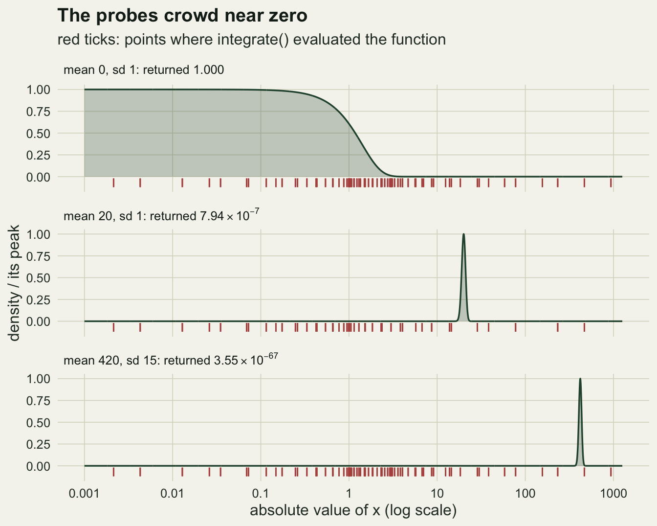
A failure map over the means and widths ecologists meet
One failing call is an anecdote. The grid below crosses nine means with six standard deviations and asks the same question of every cell: does integrate(dnorm, -Inf, Inf, mean, sd) return 1?
The grid is a choice, and the failure share is a direct function of how far out it reaches, so it needs defending in the open. The means run from 0 and 1, where a proportion or a standardised covariate lives, through 2, 5 and 10, where a log count or a logged body mass sits, to 20, 50, 100 and 420, which cover a water temperature, a plant height in centimetres, a wing length and a body length in millimetres. The standard deviations run from 1 down to 0.003. The small ones are not exotic: the integrand inside a likelihood is the product of a prior spread and a measurement kernel, and a precise measurement makes that product narrow even when the population is wide. The share is also reported for the three widest standard deviations alone, so that a reader who rejects the narrow half of the grid still gets a number.
grid_mu <- c(0, 1, 2, 5, 10, 20, 50, 100, 420)
grid_sd <- c(1, 0.3, 0.1, 0.03, 0.01, 0.003)
fail_map <- expand.grid(mu = grid_mu, sd = grid_sd)

one_cell <- function(mu, s) {
  full <- integrate(dnorm, -Inf, Inf, mean = mu, sd = s, stop.on.error = FALSE)
  half <- integrate(dnorm, 0, Inf, mean = mu, sd = s, stop.on.error = FALSE)
  subst <- integrate(function(z) dnorm(mu + s * z, mu, s) * s, -Inf, Inf)
  finite <- integrate(dnorm, mu - 8 * s, mu + 8 * s, mean = mu, sd = s)
  c(full = full$value, full_ok = full$message == "OK",
    full_abserr = full$abs.error,
    half = half$value, half_ok = half$message == "OK",
    subst = subst$value, finite = finite$value)
}
cell_res <- t(mapply(one_cell, fail_map$mu, fail_map$sd))
fail_map <- cbind(fail_map, cell_res)
fail_map$half_target <- pnorm(0, fail_map$mu, fail_map$sd, lower.tail = FALSE)

fail_map$full_wrong <- abs(fail_map$full - 1) > 0.01
fail_map$half_wrong <- abs(fail_map$half - fail_map$half_target) >
  0.01 * fail_map$half_target

n_cell      <- nrow(fail_map)
share_wrong <- mean(fail_map$full_wrong)
share_zero  <- mean(fail_map$full == 0)
n_wrong     <- sum(fail_map$full_wrong)
ok_in_fail  <- mean(fail_map$full_ok[fail_map$full_wrong] == 1)
n_not_ok    <- sum(fail_map$full_ok == 0) + sum(fail_map$half_ok == 0)
share_half  <- mean(fail_map$half_wrong)
half_agree  <- mean(fail_map$half_wrong == fail_map$full_wrong)
wide_rows   <- fail_map$sd >= 0.1
share_wide  <- mean(fail_map$full_wrong[wide_rows])
n_wide      <- sum(wide_rows)
first_fail_sd1 <- min(fail_map$mu[fail_map$sd == 1 & fail_map$full_wrong])
fail_abserr_max <- max(fail_map$full_abserr[fail_map$full_wrong])
gold_rows   <- fail_map$full_wrong & fail_map$full != 0
n_gold      <- sum(gold_rows)
n_gold_big  <- sum(fail_map$full_abserr[gold_rows] > fail_map$full[gold_rows])
default_tol <- .Machine$double.eps^0.25

near_one <- vapply(c(0.9, 1, 1.1), function(m)
  integrate(dnorm, -Inf, Inf, mean = m, sd = 0.003)$value, 0)
nz_grid <- expand.grid(mu = c(0.25, 0.5, 0.75, 1.25, 1.5, 2),
                       sd = c(0.1, 0.03, 0.01, 0.003))
nz_grid$wrong <- mapply(function(m, s)
  abs(integrate(dnorm, -Inf, Inf, mean = m, sd = s)$value - 1) > 0.01,
  nz_grid$mu, nz_grid$sd)
nz_n_fail  <- sum(nz_grid$wrong)
nz_sd_max  <- max(nz_grid$sd[nz_grid$wrong])
nz_sd3     <- sum(nz_grid$wrong[nz_grid$sd == 0.003])

worst_subst  <- max(abs(fail_map$subst - 1))
worst_finite <- max(abs(fail_map$finite - 1))

hn_sigma <- c(1, 10, 50, 100, 500)
hn_err <- vapply(hn_sigma, function(sg) {
  num <- integrate(function(r) exp(-r^2 / (2 * sg^2)), 0, Inf)$value
  abs(num / (sg * sqrt(pi / 2)) - 1)
}, 0)
hn_worst <- max(hn_err)

tight_call <- integrate(dnorm, -Inf, Inf, mean = 420, sd = 15,
                        rel.tol = 1e-10, subdivisions = 1000L)
tight_val <- tight_call$value
tight_msg <- tight_call$message

help_20000 <- integrate(dnorm, 0, 20000)$value
help_inf   <- integrate(dnorm, 0, Inf)$value
Of the 54 cells, 35 come back more than 1 per cent wrong, a share of 0.648, and 0.519 of all cells come back as exactly 0. These calls, too, were made with stop.on.error = FALSE: under the default a failure the routine detects stops with an error, and the OK share below could not be anything but 1. Among the failures, the share whose message is "OK" is 1.000, and the number of cells anywhere on the grid, whole line or half line, with any other message is 0. The informative fact is that the routine flagged nothing: its own error test was satisfied in every one of these cells. The largest absolute error integrate() reported for a failing cell was \(1.55 \times 10^{-5}\), and that small number is no comfort. In 6 of the 7 failing cells that are not exactly 0, the reported error is larger than the value itself. It passes because the default abs.tol equals rel.tol, .Machine$double.eps^0.25 or \(1.22 \times 10^{-4}\), and it is an absolute tolerance: an integral smaller than that can be accepted whatever its relative error. Restricted to the 27 cells with a standard deviation of 0.1 or more, the failure share is 0.519. At a standard deviation of 1 the first mean that fails is 20.
The all-green column at a mean of 1 is luck rather than safety: x = 1 is where the transformation puts the centre point of the rule’s first pass. At a standard deviation of 0.003, means of 0.9, 1 and 1.1 return \(1.09 \times 10^{-16}\), 1.000 and \(3.18 \times 10^{-48}\).
The trap is not confined to doubly infinite limits. Integrating the same densities over the half line from 0 to infinity, against the exact target from pnorm(), 0.648 of cells are more than 1 per cent wrong, and the half line and the whole line agree on which cells fail in 1.000 of the grid. What does not fail is a half-normal detection function with its scale in metres, the most common detection function in distance sampling, over the same half line: at a scale of 1, 10, 50, 100 and 500 m the worst relative error is \(2.58 \times 10^{-10}\). Its mass sits at zero, where the probes are.
fail_map$verdict <- ifelse(!fail_map$full_wrong, "within 1 per cent of 1",
                    ifelse(fail_map$full == 0, "exactly 0", "wrong, not zero"))
fail_map$verdict <- factor(fail_map$verdict,
  levels = c("within 1 per cent of 1", "wrong, not zero", "exactly 0"))
fail_map$lab <- ifelse(fail_map$full == 0, "0",
                ifelse(fail_map$full_wrong,
                       sub("e(.*)", " %*% 10^\\1", sprintf("%.0e", fail_map$full)), "1"))
fail_map$lab <- gsub("\\^([+-]?)0*([0-9])", "^\\1\\2", fail_map$lab)  # 10^-07 -> 10^-7

ggplot(fail_map, aes(factor(mu), factor(sd, levels = grid_sd))) +
  geom_tile(aes(fill = verdict), colour = te_paper, linewidth = 1) +
  geom_text(aes(label = lab), size = 2.9, parse = TRUE,
            colour = ifelse(fail_map$verdict == "within 1 per cent of 1",
                            te_paper, te_ink)) +
  scale_fill_manual(values = c(te_forest, te_gold, te_rust), name = NULL,
                    drop = FALSE) +
  labs(x = "mean", y = "standard deviation",
       title = "Every failure reports OK",
       subtitle = sprintf("cell text: the value returned; no error raised, message OK in all %d cells", n_cell)) +
  theme_datasheet() +
  theme(legend.position = "bottom", panel.grid.major = element_blank())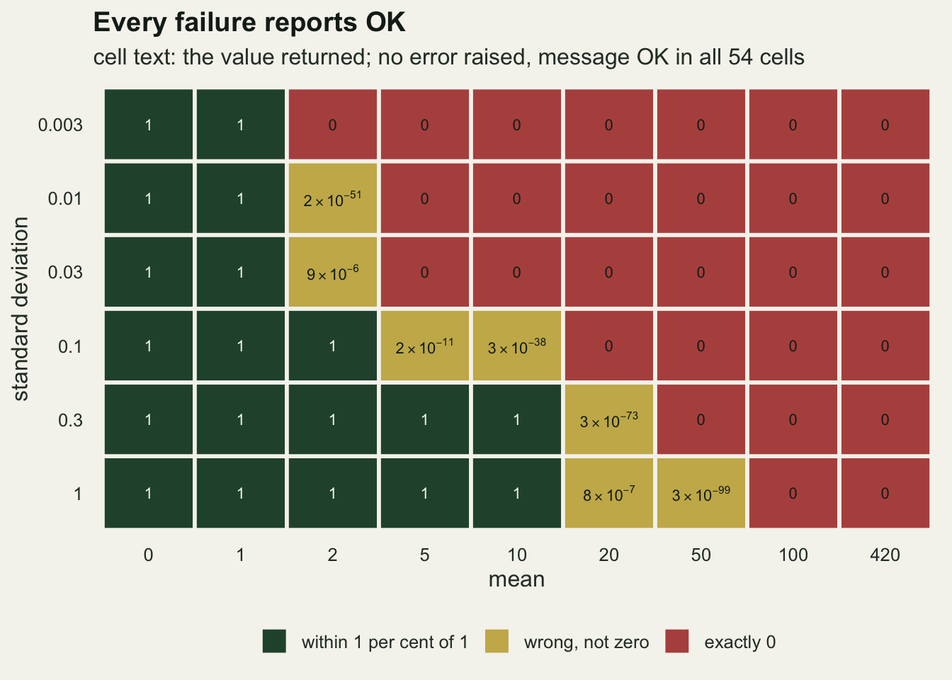
The help page points the other way
The help page warns in general terms, then points the reader the wrong way. The second example in ?integrate is integrate(dnorm, -Inf, Inf), the call that fails above as soon as the mean moves. Further down, the Examples block shows the infinite limit as the repair for a failure on a wide finite range:
## integrate can fail if misused
integrate(dnorm, 0, 20000) ## fails on many systems
integrate(dnorm, 0, Inf)   ## works
On this machine the first returns 0 and the second 0.500000. The Note section of the page makes two points that matter here, in this order. The first is the general warning: “If the function is approximately constant (in particular, zero) over nearly all its range it is possible that the result and error estimate may be seriously wrong.” The second is the advice those two example lines act out: “When integrating over infinite intervals do so explicitly, rather than just using a large number as the endpoint. This increases the chance of a correct answer - any function whose integral over an infinite interval is finite must be near zero for most of that interval.” For a density centred at zero the advice is right. A density at 420 mm is near zero over nearly all of the real line as well, which is the first warning’s case, and the explicit infinite limit is exactly the call that misses it. The rule to take away is about where the mass sits relative to the points the routine tries first, not about whether the limits are finite.
Two repairs, and which gives way first
On the grid above, both of the usual repairs are exact. Substituting the standardised variable, so that the routine integrates over z with x equal to the mean plus sd times z, gives a worst absolute error of \(2.06 \times 10^{-10}\); finite limits at the mean plus and minus 8 standard deviations give \(2.08 \times 10^{-12}\). That comparison flatters the substitution, though: for a single normal density the substituted integrand is the standard normal in every cell, so its exactness there is a tautology. The test that separates them is the integrand the fish likelihood actually needs.
For one fish with recorded length w, the integrand over its true length x is the measurement kernel, a normal density for w centred on x with sd equal to the measurement error, times the population density of x. Without the logistic term its integral has a closed form, a normal density for w with variance equal to the sum of the two variances, which makes it a benchmark. Both repairs are built from the population scale: the substitution centres on the population mean and scales by the population sd, and the finite limits sit 8 population sds either side. As the measurement error shrinks, the integrand becomes a narrow spike somewhere inside that range, and the question is which repair loses it first. A third route centres and scales on the integrand itself, on the mean and sd of the true length given that fish’s record, which is the idea behind the adaptive Gauss-Hermite rule of Liu and Pierce.
pop_mu <- 420
pop_sd <- 15
me_grid <- c(8, 4, 2, 1.4, 1, 0.7, 0.5, 0.35, 0.25, 0.1)
w_offsets <- c(-2, -1, 0, 0.5, 1, 2)

repair_cell <- function(me_sd, w_rec) {
  f_raw  <- function(x) dnorm(w_rec, x, me_sd) * dnorm(x, pop_mu, pop_sd)
  target <- dnorm(w_rec, pop_mu, sqrt(pop_sd^2 + me_sd^2))
  post_sd <- 1 / sqrt(1 / pop_sd^2 + 1 / me_sd^2)
  post_mu <- post_sd^2 * (w_rec / me_sd^2 + pop_mu / pop_sd^2)
  r_sub <- integrate(function(z) f_raw(pop_mu + pop_sd * z) * pop_sd, -Inf, Inf,
                     stop.on.error = FALSE)
  r_fin <- integrate(f_raw, pop_mu - 8 * pop_sd, pop_mu + 8 * pop_sd,
                     stop.on.error = FALSE)
  r_own <- integrate(function(z) f_raw(post_mu + post_sd * z) * post_sd,
                     -Inf, Inf, stop.on.error = FALSE)
  c(sub = abs(r_sub$value / target - 1), fin = abs(r_fin$value / target - 1),
    own = abs(r_own$value / target - 1),
    msg_ok = all(c(r_sub$message, r_fin$message, r_own$message) == "OK"))
}

repair_tab <- do.call(rbind, lapply(me_grid, function(me_sd) {
  cells <- vapply(pop_mu + pop_sd * w_offsets,
                  function(w_rec) repair_cell(me_sd, w_rec), numeric(4))
  data.frame(me_sd = me_sd, ratio = pop_sd / me_sd,
             sub = max(cells["sub", ]), fin = max(cells["fin", ]),
             own = max(cells["own", ]), all_ok = all(cells["msg_ok", ] == 1))
}))

fin_first <- max(repair_tab$me_sd[repair_tab$fin > 0.01])
sub_first <- max(repair_tab$me_sd[repair_tab$sub > 0.01])
own_worst <- max(repair_tab$own)
repair_all_ok <- all(repair_tab$all_ok)
fin_ratio <- pop_sd / fin_first
sub_ratio <- pop_sd / sub_first
With a population sd of 15 mm, the finite limits first miss by more than 1 per cent at a measurement error of 1.0 mm, a population-to-error ratio of 15. The prior-centred substitution survives a little longer and first fails at 0.7 mm, a ratio of 21.4. The two are one step apart on this grid, and which goes first depends on the 8 sd width and on the recorded lengths tried, so the order is no ranking of the two. Below that both return essentially nothing. Centring and scaling on the integrand’s own location and width is exact to a worst relative error of \(2.06 \times 10^{-10}\) across the whole range, including a measurement error of 0.10 mm. With stop.on.error = FALSE again, the message was "OK" in every one of these calls, failures included (the check over all of them returns TRUE).
So the answer to which repair to recommend is neither of the two usual ones. Both borrow their location and scale from the population, and both fail once the measurement is precise enough that one fish’s integrand is much narrower than the population it came from. A calliper error of a millimetre on fish that vary by 15 mm is enough to break the finite limits. The repair that holds is to put the routine’s origin on the integrand’s own centre and its unit on the integrand’s own width. For the Gaussian part of this model both are available in closed form, and the logistic term only tilts the integrand gently on the scale of one over the slope; for a model where they are not, a few Newton steps to the mode of each integrand give them.
err_floor <- 1e-14
repair_long <- rbind(
  data.frame(ratio = repair_tab$ratio, err = repair_tab$fin,
             route = "finite limits at population mean +/- 8 sd"),
  data.frame(ratio = repair_tab$ratio, err = repair_tab$sub,
             route = "substitution on the population scale"),
  data.frame(ratio = repair_tab$ratio, err = repair_tab$own,
             route = "substitution on the integrand's own scale"))
repair_long$err <- pmax(repair_long$err, err_floor)

ggplot(repair_long, aes(ratio, err, colour = route)) +
  geom_hline(yintercept = 0.01, linetype = "dashed", colour = te_body,
             linewidth = 0.5) +
  geom_line(linewidth = 0.9) +
  geom_point(size = 2.2) +
  scale_x_log10() +
  scale_y_log10(breaks = 10^c(-14, -10, -6, -2, 0),
                labels = expression(10^-14, 10^-10, 10^-6, 0.01, 1)) +
  scale_colour_manual(values = c(te_rust, te_gold, te_forest), name = NULL) +
  guides(colour = guide_legend(ncol = 1)) +
  labs(x = "population sd / measurement error sd (log scale)",
       y = "worst relative error (log scale)",
       title = "Borrowed scales fail as measurement sharpens",
       subtitle = expression("dashed: 1 per cent; errors below " * 10^-14 * " drawn at the floor")) +
  theme_datasheet() +
  theme(legend.position = "bottom")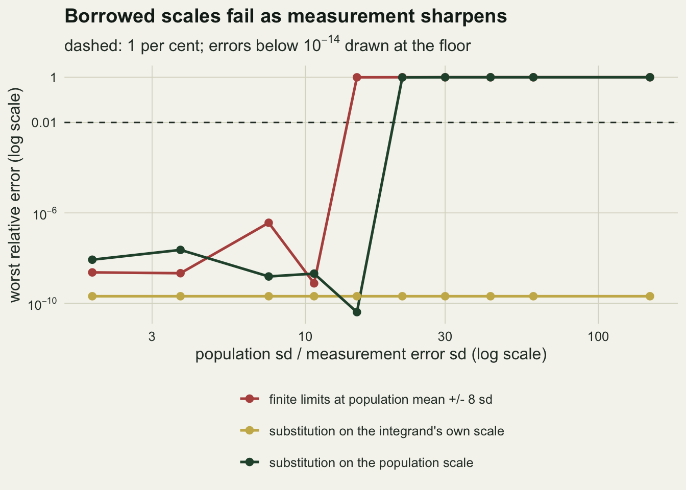
A likelihood the failure breaks
A failure map on its own is a curiosity. The question for an analysis is whether the misses survive into an estimate, and the only fair way to ask it is to fit the same data twice. Two independent sets of simulations, one per route, would bury a difference of this kind under sampling noise; fitting both routes to the same dataset from the same start differences that noise out, so the comparison below is paired throughout.
The model is classical measurement error in body length. True length x is normal with mean mu and sd sx in millimetres, the recorded length is w, x plus normal error with sd su, and maturity follows a logistic regression on centred true length with intercept -0.4 and slope 0.08 per mm, for 180 fish. The likelihood for one fish integrates the logistic probability of its maturity state, times the measurement kernel, times the population density, over true length; the population parameters and su are treated as known so that only the intercept and slope are estimated, which keeps the computation the only thing that differs. The raw route integrates over x in millimetres from minus to plus infinity. The standardised route integrates the same function over z, with x equal to mu plus sx times z. Both are minimised by Nelder-Mead from the start (0, 0) with the same control settings, and a naive logistic regression on the recorded length is carried along as the reference the integral exists to improve on. The regimes and the 25 datasets per regime, with their seeds, were fixed before anything ran.
n_fish  <- 180
b0_true <- -0.4
b1_true <- 0.08
n_rep   <- 25
regimes <- data.frame(mu = c(420, 420, 250), sx = c(15, 25, 20),
                      su = c(8, 10, 12))
regimes$label <- sprintf("mean %g, sd %g, error %g mm",
                         regimes$mu, regimes$sx, regimes$su)
nm_control <- list(maxit = 220, reltol = 1e-9)

fit_pair <- function(seed, mu_x, sx, su, own_only = FALSE) {
  set.seed(seed)
  x_true <- rnorm(n_fish, mu_x, sx)
  w_rec  <- x_true + rnorm(n_fish, 0, su)
  y_mat  <- rbinom(n_fish, 1, plogis(b0_true + b1_true * (x_true - mu_x)))
  sgn    <- 2 * y_mat - 1
  post_sd <- 1 / sqrt(1 / sx^2 + 1 / su^2)
  post_mu <- post_sd^2 * (w_rec / su^2 + mu_x / sx^2)

  obs_int <- function(th, i, route, soe = TRUE) {
    kern <- function(xx) plogis(sgn[i] * (th[1] + th[2] * (xx - mu_x))) *
      dnorm(w_rec[i], xx, su) * dnorm(xx, mu_x, sx)
    if (route == "raw") {
      integrate(kern, -Inf, Inf, stop.on.error = soe)
    } else if (route == "std") {
      integrate(function(z) kern(mu_x + sx * z) * sx, -Inf, Inf,
                stop.on.error = soe)
    } else {
      integrate(function(z) kern(post_mu[i] + post_sd * z) * post_sd,
                -Inf, Inf, stop.on.error = soe)
    }
  }
  all_int <- function(th, route) {
    vapply(seq_len(n_fish), function(i) obs_int(th, i, route)$value, 0)
  }
  # value, reported abs.error and message per fish, with failures that the
  # routine detects returned as messages instead of errors
  int_detail <- function(th, route) {
    t(vapply(seq_len(n_fish), function(i) {
      r <- obs_int(th, i, route, soe = FALSE)
      c(value = r$value, abs_err = r$abs.error, ok = r$message == "OK")
    }, numeric(3)))
  }
  err_flag <- function(d) mean(d[, "value"] == 0 | d[, "abs_err"] > 0.01 * d[, "value"])
  nll <- function(th, route) -sum(log(pmax(all_int(th, route), 1e-300)))

  if (own_only) {
    fit_own <- optim(c(0, 0), nll, route = "own", method = "Nelder-Mead",
                     control = nm_control)
    return(fit_own$par[2])
  }
  fit_std <- optim(c(0, 0), nll, route = "std", method = "Nelder-Mead",
                   control = nm_control)
  fit_raw <- optim(c(0, 0), nll, route = "raw", method = "Nelder-Mead",
                   control = nm_control)
  naive <- unname(coef(glm(y_mat ~ I(w_rec - mu_x), family = binomial))[2])

  det_raw <- int_detail(fit_raw$par, "raw")
  det_std <- int_detail(fit_std$par, "std")
  int_raw_fit <- det_raw[, "value"]
  int_own_fit <- all_int(fit_raw$par, "own")
  c(raw = fit_raw$par[2], std = fit_std$par[2], naive = naive,
    conv_raw = fit_raw$convergence, conv_std = fit_std$convergence,
    zero_share = mean(int_raw_fit == 0),
    log10_ratio = median(log10(pmax(int_raw_fit, 1e-300) / int_own_fit)),
    gap_raw = fit_raw$value + sum(log(pmax(int_own_fit, 1e-300))),
    gap_std = fit_std$value - nll(fit_std$par, "own"),
    ok_share = mean(det_raw[, "ok"]),
    flag_raw = err_flag(det_raw), flag_std = err_flag(det_std))
}

pair_res <- do.call(rbind, lapply(seq_len(nrow(regimes)), function(k) {
  out <- t(vapply(1000 * k + seq_len(n_rep), fit_pair, numeric(12),
                  mu_x = regimes$mu[k], sx = regimes$sx[k],
                  su = regimes$su[k]))
  data.frame(regime = regimes$label[k], dataset = seq_len(n_rep), out)
}))
pair_res$regime <- factor(pair_res$regime, levels = regimes$label)
pair_res$rel_diff <- (pair_res$raw - pair_res$std) / abs(pair_res$std)
pair_res$naive_closer <- abs(pair_res$naive - pair_res$std) <
  abs(pair_res$raw - pair_res$std)

by_regime <- function(v, fun) as.numeric(tapply(v, pair_res$regime, fun))
med_raw   <- by_regime(pair_res$raw, median)
min_raw   <- by_regime(pair_res$raw, min)
max_raw   <- by_regime(pair_res$raw, max)
med_std   <- by_regime(pair_res$std, median)
med_naive <- by_regime(pair_res$naive, median)
med_rel   <- by_regime(pair_res$rel_diff, median)
med_abs_rel <- by_regime(abs(pair_res$rel_diff), median)
share_big <- by_regime(abs(pair_res$rel_diff) > 0.30, mean)
n_big     <- by_regime(abs(pair_res$rel_diff) > 0.30, sum)
# exact bootstrap percentile interval for a median of an odd number of
# values: the resampled median is at most v[k] when at least (n + 1) / 2 of
# the n draws are, a binomial count with probability k / n
boot_ci <- vapply(levels(pair_res$regime), function(r) {
  v <- sort(abs(pair_res$rel_diff[pair_res$regime == r]))
  n <- length(v)
  cdf <- pbinom((n - 1) / 2, n, seq_len(n) / n, lower.tail = FALSE)
  c(v[which(cdf >= 0.025)[1]], v[which(cdf >= 0.975)[1]])
}, numeric(2))
conv_raw  <- by_regime(pair_res$conv_raw == 0, mean)
n_maxit   <- by_regime(pair_res$conv_raw == 1, sum)
flag_raw_med <- by_regime(pair_res$flag_raw, median)
flag_std_med <- by_regime(pair_res$flag_std, median)
flag_std_max <- max(pair_res$flag_std)
conv_std  <- by_regime(pair_res$conv_std == 0, mean)
neg_raw   <- by_regime(pair_res$raw < 0, sum)
naive_win <- by_regime(pair_res$naive_closer, mean)
zero_med  <- by_regime(pair_res$zero_share, median)
ratio_med <- by_regime(pair_res$log10_ratio, median)
gap_raw_med <- by_regime(pair_res$gap_raw, median)
gap_raw_min <- min(pair_res$gap_raw)
gap_std_max <- max(abs(pair_res$gap_std))
gap_std_med <- median(abs(pair_res$gap_std))
gap_fold <- log10(gap_raw_min / gap_std_max)
n_big_regimes <- sum(med_abs_rel > 0.30)
n_own <- 3
# refit the integrand-centred route only; the standardised slopes of the
# same datasets are already in pair_res
own_check <- do.call(rbind, lapply(seq_len(nrow(regimes)), function(k) {
  own <- vapply(1000 * k + seq_len(n_own), fit_pair, 0,
                mu_x = regimes$mu[k], sx = regimes$sx[k], su = regimes$su[k],
                own_only = TRUE)
  cbind(std = pair_res$std[as.integer(pair_res$regime) == k &
                             pair_res$dataset <= n_own], own = own)
}))
own_rel_max <- max(abs(own_check[, "std"] - own_check[, "own"]) /
                     abs(own_check[, "own"]))
ok_share_min <- min(pair_res$ok_share)
ratio_lo <- min(regimes$sx / regimes$su)
ratio_hi <- max(regimes$sx / regimes$su)

canary <- vapply(seq_len(nrow(regimes)), function(k)
  integrate(dnorm, -Inf, Inf, mean = regimes$mu[k], sd = regimes$sx[k])$value, 0)
# a canary that passes: fish of about 10 cm, sd 1 cm, measured to 0.3 mm
canary_pass   <- integrate(dnorm, -Inf, Inf, mean = 10, sd = 1)$value
canary_prod   <- integrate(function(x) dnorm(10.5, x, 0.03) * dnorm(x, 10, 1),
                           -Inf, Inf)$value
canary_target <- dnorm(10.5, 10, sqrt(1 + 0.03^2))
The standardised route recovers median slopes of 0.0806, 0.0821 and 0.0840 per mm in the three regimes, against a true 0.08, and converges with code 0 in 1.00, 1.00 and 1.00 of datasets. That is the fit the student wanted.
The raw route, on the same datasets from the same start, gives median slopes of +0.0332, +0.0010 and +0.0060, with ranges across datasets of -0.1129 to +0.1133, -0.4396 to +0.1627, and +0.0029 to +0.0372. The slope comes out negative in 10, 11 and 0 of the 25 datasets. Paired dataset by dataset, the raw estimate minus the standardised one, as a fraction of the standardised one, has a median of -0.546, -0.992 and -0.930, and a median magnitude of 0.730, 0.998 and 0.930. Resampling the 25 datasets, the exact 95 per cent bootstrap percentile intervals for those medians run from 0.338 to 2.093, 0.930 to 1.321 and 0.919 to 0.938; the first regime, where the raw route lands in very different places, is the one a different set of seeds would move most. The two routes differ by more than 30 per cent of the standardised estimate in 20, 24 and 25 of the 25 datasets.
Little in the output flags it. At the raw fits’ own parameters, recomputed with stop.on.error = FALSE, the smallest share of per-fish integrals returning the message "OK" in any dataset is 1.000: the routine’s own error test passed on every fish. The raw fits converge with code 0 in 1.00, 0.76 and 1.00 of datasets. The only signal is the 6 fits in the second regime that stopped at the iteration limit (code 1), and an iteration limit says nothing about the integrals. And the broken fit is worse than doing nothing: the naive regression on recorded length, which ignores the measurement error altogether and is known to be attenuated, gives median slopes of 0.0588, 0.0633 and 0.0542, and lands closer to the correct estimate than the raw route does in 0.80, 0.96 and 1.00 of datasets.
pair_res$rank <- ave(pair_res$std, pair_res$regime,
                     FUN = function(v) rank(v, ties.method = "first"))
pair_long <- rbind(
  data.frame(pair_res[, c("regime", "rank")], slope = pair_res$std,
             route = "integrated, standardised"),
  data.frame(pair_res[, c("regime", "rank")], slope = pair_res$raw,
             route = "integrated, raw mm scale"),
  data.frame(pair_res[, c("regime", "rank")], slope = pair_res$naive,
             route = "naive glm on recorded length"))
pair_long$route <- factor(pair_long$route,
  levels = c("integrated, standardised", "integrated, raw mm scale",
             "naive glm on recorded length"))

ggplot(pair_long, aes(rank, slope)) +
  geom_hline(yintercept = b1_true, linetype = "dashed", colour = te_body,
             linewidth = 0.5) +
  geom_hline(yintercept = 0, colour = te_line, linewidth = 0.6) +
  geom_segment(data = pair_res, aes(x = rank, xend = rank, y = std, yend = raw),
               colour = "grey60", linewidth = 0.4) +
  geom_point(aes(colour = route, shape = route), size = 1.9) +
  facet_wrap(~ regime, ncol = 1, scales = "free_y") +
  scale_colour_manual(values = c(te_forest, te_rust, te_gold), name = NULL) +
  scale_shape_manual(values = c(16, 17, 15), name = NULL) +
  guides(colour = guide_legend(ncol = 1), shape = guide_legend(ncol = 1)) +
  labs(x = "dataset, ordered by the standardised estimate",
       y = "slope per mm",
       title = "Same data, same start, different computation",
       subtitle = "dashed: the true slope 0.08") +
  theme_datasheet() +
  theme(legend.position = "bottom",
        strip.text = element_text(colour = te_ink, hjust = 0))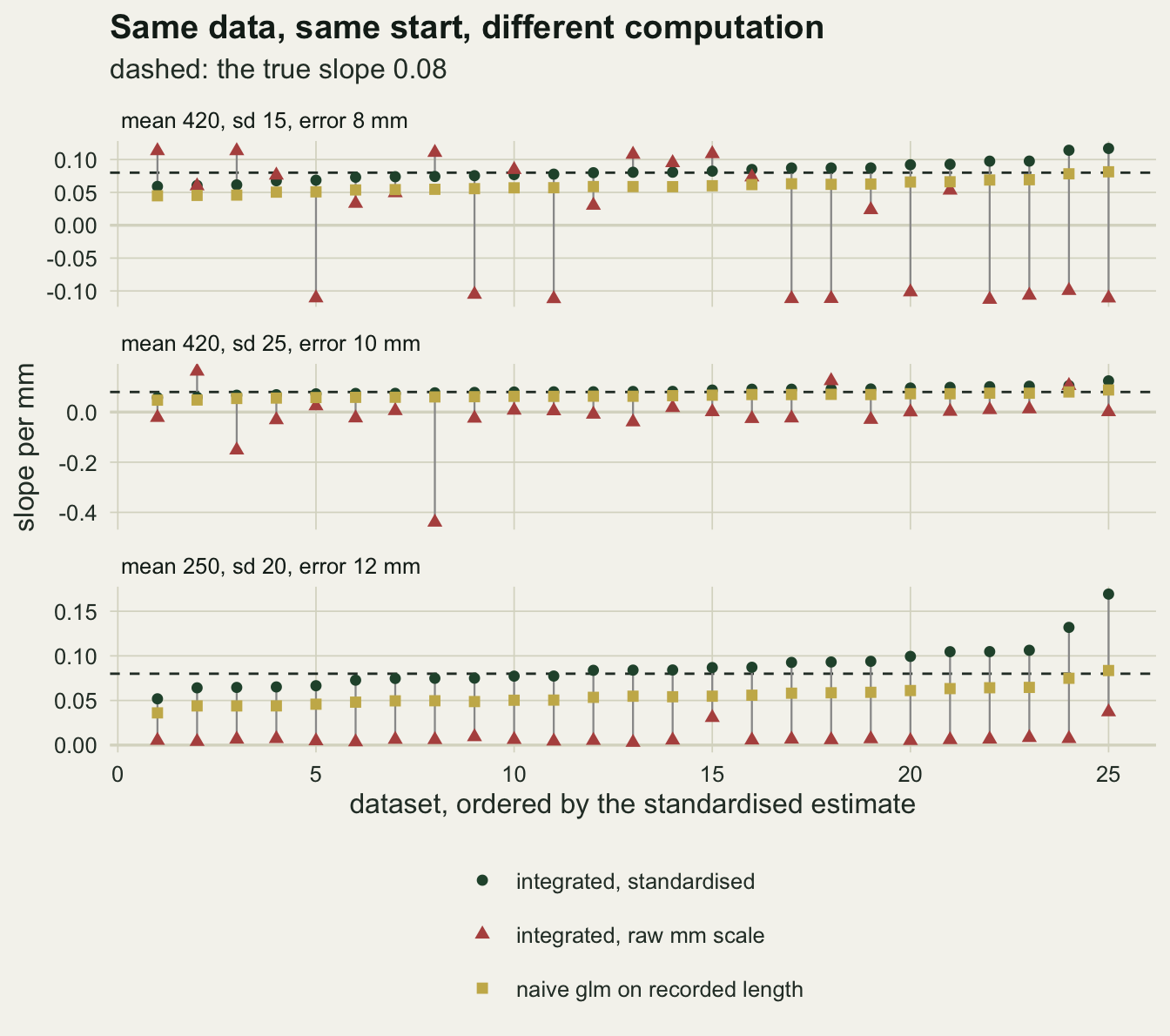
Why a check for zeros is not enough
The obvious diagnostic is to look for integrals that came back as exactly 0 and treat any as a red flag. It does not work well here. At the raw route’s own fitted parameters, the median share of per-fish integrals that are exactly 0 is 0.072, 0.000 and 0.000 in the three regimes. Most of the damage is done by integrals that are not zero but are wrong: against the integrand-centred route at the same parameters, the median per-fish log10 ratio of raw to correct is -9.2, -8.9 and -60.4. The raw integrals are positive numbers many orders of magnitude too small, and the optimiser is doing its honest best on a surface made of them.
The reported absolute error does better, if it is read against the value rather than on its own. A rule that flags a fish whose integral is 0 or whose reported error exceeds 1 per cent of its value flags a median share of 1.00, 0.71 and 0.00 of fish at the raw fits in the three regimes. That catches the first two regimes and misses the third, where the error estimate shrinks along with the wrong value. On the standardised fits the same rule flags a median of 0.04, 0.13 and 0.12 of fish, and up to 0.18 in one dataset, so a flag marks a fish to look at rather than a broken fit. It is cheap and worth running, and it is not the check that clears a fit.
Two checks do catch it here, and both are cheap enough to run after every fit. The first is to recompute the log-likelihood at the fitted parameters by a second route that centres differently, here the integrand-centred one, and compare. For the raw fits the negative log-likelihood reported by optim() exceeds the recomputed one by a median of 12643, 27245 and 24723 log-likelihood units, and by at least 4373 in every dataset. For the standardised fits the median disagreement is \(5.72 \times 10^{-4}\) units and the largest is 0.169. That is not zero, because the population-centred substitution is itself slightly off for a fish whose integrand sits far from the population centre, a milder form of the failure in the previous section; but the smallest raw gap is 4.4 orders of magnitude larger than the largest standardised one. A likelihood that changes when the variable of integration is merely shifted is not being computed. The second check is cruder and needs no second route: integrate the population density on its own, with the same call, and see whether it returns 1. For the three regimes integrate(dnorm, -Inf, Inf, mean = mu, sd = sx) returns \(3.55 \times 10^{-67}\), \(2.06 \times 10^{-24}\) and \(1.42 \times 10^{-16}\). This check is one-sided: a population density that integrates to 1 says nothing about the narrower product integrand, so a pass is no clearance. For fish of about 10 cm with a standard deviation of 1 cm, measured to 0.3 mm, the population density returns 1.000000, and the integrand for a fish recorded at 10.5 cm returns 0 against an exact 0.352.
diag_df <- rbind(
  data.frame(regime = pair_res$regime, gap = abs(pair_res$gap_std),
             route = "integrated, standardised"),
  data.frame(regime = pair_res$regime, gap = abs(pair_res$gap_raw),
             route = "integrated, raw mm scale"))
diag_df$gap <- pmax(diag_df$gap, 1e-12)
diag_df$route <- factor(diag_df$route, levels = c("integrated, standardised",
                                                  "integrated, raw mm scale"))

ggplot(diag_df, aes(gap, regime, colour = route)) +
  geom_point(position = position_jitter(height = 0.18, width = 0, seed = 7),
             size = 1.8, alpha = 0.85) +
  scale_x_log10(breaks = 10^c(-12, -8, -4, 0, 4),
                labels = expression(10^-12, 10^-8, 10^-4, 1, 10^4)) +
  scale_colour_manual(values = c(te_forest, te_rust), name = NULL) +
  labs(x = "absolute gap in negative log-likelihood (log scale)", y = NULL,
       title = "A shifted variable should not move the likelihood",
       subtitle = expression("one point per dataset and route; gaps below " * 10^-12 * " drawn at the floor")) +
  theme_datasheet() +
  theme(legend.position = "bottom", plot.title.position = "plot")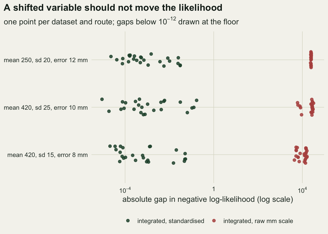
What to report
State the variable of integration and how it was centred and scaled, in the methods, the way a mesh size or a number of quadrature nodes would be stated. “The likelihood integrates over true length with integrate()” is not a description of the computation; “over the standardised true length, centred on each fish’s conditional mean” is.
Report a check of the integral against something exact. For a measurement-error or random-effects likelihood the population density on its own integrates to 1, and a line of code shows whether the call can see even that; a pass is necessary, not sufficient, and the second-route check below is the one that clears a fit. Where the model has a closed-form special case, such as the Gaussian part here, report the worst relative error of the routine against it over the range of the data.
Report the log-likelihood at the fitted parameters from a second, differently centred route, and the gap between the two. The convergence code and the message describe the routine’s view of its own work: in this post the message was OK on every fish and the code was 0 on most fits that were wrong by most of the estimate. The reported absolute error helps only when it is read against the value, and even then it caught two regimes of three.
If a naive estimate is available, report it next to the corrected one. A correction for measurement error should move the slope away from zero by an amount the reliability ratio makes plausible. A corrected slope that lands nearer zero than the naive one, or on the other side of it, is a computation problem until shown otherwise.
Honest limits
The failure map uses one integrand, the normal density, and one grid. The share of failing cells is a function of where the grid reaches, as the section defending it says, and a grid confined to means near zero finds failures only at narrow widths: over means from 0.25 to 2 and standard deviations from 0.1 down to 0.003, 7 of 24 cells fail, 5 of them at 0.003 and none at a standard deviation above 0.03. The claim that survives any grid is the qualitative one: the routine’s first probes sit near the origin on the scale of the argument, and a narrow mass far from them can be missed and reported as OK.
The behaviour depends on the QUADPACK implementation in R 4.3.3 and on the default tolerances. A tighter rel.tol or a larger subdivisions should not help when the probes see nothing, since a subinterval on which both rules return zero shows no error to reduce, and the one check made agrees: the fish-length call with rel.tol = 1e-10 and subdivisions = 1000 returns \(3.55 \times 10^{-67}\) with message "OK". No other settings or R versions were tested.
The downstream model treats the population mean and sd of true length, and the measurement error sd, as known. In a real analysis they are estimated, usually from replicate measurements, and the uncertainty in them adds to the uncertainty in the slope. That changes the size of the standard errors, not the computational point. Stefanski and Carroll’s conditional score avoids the integral altogether for a logistic model with normal measurement error, and Carroll and colleagues give the structural likelihood used here in full; neither is compared with this fit.
Only three regimes were run, with 25 datasets each and population-to-error ratios between 1.67 and 2.50. At those ratios the prior-centred substitution is close to exact, though not exact, as the next paragraph says. The section on repairs shows it failing once the ratio reaches 21.4, which is the case of a precise instrument on a variable population; a fit in that range would need the integrand-centred route, and none was fitted here.
The paired reference is the standardised route, which the diagnostic above shows is not exact either: its log-likelihood differs from the integrand-centred one by up to 0.169 units. The integrand-centred route was fitted to the first 3 datasets of each regime as a check, and there the standardised slope differs from it by at most 0.0003 of its value, against paired raw gaps of most of the estimate; the other datasets were not refitted, so the standardised slopes stay the reference because that design was fixed before the run, not because they are the best available.
Nelder-Mead from a fixed start is a single optimiser run. A different start or a gradient method might land the raw route elsewhere, and in the first regime it lands in very different places across datasets already. That instability is part of the finding, not a correction to it: a surface made of wrong integrals has no right answer to converge to.
References
Piessens R, de Doncker-Kapenga E, Ueberhuber CW, Kahaner DK 1983 QUADPACK: A Subroutine Package for Automatic Integration (ISBN 978-3-540-12553-2)
Liu Q, Pierce DA 1994 Biometrika 81(3):624-629 (10.1093/biomet/81.3.624)
Stefanski LA, Carroll RJ 1987 Biometrika 74(4):703-716 (10.1093/biomet/74.4.703)
Carroll RJ, Ruppert D, Stefanski LA, Crainiceanu CM 2006 Measurement Error in Nonlinear Models, 2nd edition (ISBN 978-1-58488-633-4)