Fat tails and accelerating spread

An invasion front with a fat-tailed dispersal kernel never settles at a constant speed. Simulating and measuring accelerating spread in R with ggplot2.

An invasive annual holds 40 metres of one bank of a lowland river. The catchment partnership has three years of survey money and one question: where will the leading edge be in twenty years, and in forty. Somebody has already done the hard part and fitted a dispersal kernel to a marked seed recovery, so the growth rate and the median jump are both in hand. What remains looks like arithmetic.

It is not. Two kernels that agree on the median jump, on the growth rate and on every seed the survey recovered can produce forecasts that differ by a multiple rather than a margin, and they can disagree about something more basic than the answer: whether the question has one. A front driven by a thin-tailed kernel travels at an asymptotic speed, so the twenty year and forty year answers are the same number twice. A front driven by a fat-tailed kernel has no asymptotic speed at all. It accelerates, without limit, for as long as the model is run. This tutorial simulates both on the same grid and measures the difference: the exponent of the front trajectory, the integral that separates the two cases, and the number of years of forecast the choice of kernel family is worth.

Two earlier tutorials set this up. Fat-tailed dispersal kernels measures the tail itself: thin and fat families fitted to one seed rain agree in the bulk and separate by orders of magnitude past the data. The speed of an invasion front takes a thin-tailed kernel and computes the speed in closed form from the moment generating function. The post you are reading is what happens when that closed form has nothing to compute: the tail is fat, the moment generating function diverges, and the front runs away from its own average speed.

library(ggplot2)

te_pal <- list(forest = "#275139", green = "#2f8f63", sage = "#93a87f",
               clay = "#b5534e", gold = "#cda23f", line = "#dad9ca",
               ink = "#16241d", paper = "#f5f4ee")

theme_te <- function() {
  theme_minimal(base_size = 12) +
    theme(panel.grid.minor = element_blank(),
          panel.grid.major = element_line(colour = "#e7e6dc"),
          plot.background = element_rect(fill = "#f5f4ee", colour = NA),
          panel.background = element_rect(fill = "#f5f4ee", colour = NA),
          plot.title = element_text(face = "bold", colour = te_pal$ink),
          axis.title = element_text(colour = "#2c3a31"))
}

Four kernels that agree about the median jump

The kernel is a probability distribution for one generation’s displacement along the corridor, so the model is one dimensional: distance up or down the bank. Four families, each given the same median absolute displacement of 8 metres, so that the bulk of the dispersal is held fixed and only the far tail varies.

The Gaussian falls off like the exponential of minus a square. The stretched exponential falls off like the exponential of minus a fractional power, and the two versions used here take that power to be 0.5 and 0.4: still exponential in form, but slow enough to count as fat, which has a precise meaning reached in a later section. The power law kernel is a scaled Student t with three degrees of freedom, whose density falls off as distance to the minus four, so the far tail decays polynomially rather than exponentially.

Each family is defined by the survival function of the absolute displacement, the probability of a jump longer than a given distance, rather than by the density. There are two numerical reasons and both matter later. The discrete kernel is then built by integrating the density over each grid cell rather than sampling it at the cell centre, and the tail probabilities are computed in the upper tail throughout. Building the same weights by differencing a distribution function silently deletes the whole kernel tail past the distance where the distribution function rounds to one, which for the stretched exponential with shape 0.5 happens at about four kilometres.

med_jump <- 8

kern_gauss <- function(m) {
  sg <- m / qnorm(0.75)
  list(surv = function(r) 2 * pnorm(r, 0, sg, lower.tail = FALSE),
       dens = function(z) dnorm(z, 0, sg), par = c(scale = sg))
}
kern_stretch <- function(m, cc) {
  aa <- m / qgamma(0.5, shape = 1 / cc)^(1 / cc)
  list(surv = function(r) pgamma((r / aa)^cc, shape = 1 / cc, lower.tail = FALSE),
       dens = function(z) (cc / (2 * aa * gamma(1 / cc))) * exp(-(abs(z) / aa)^cc),
       par = c(scale = aa, shape = cc))
}
kern_power <- function(m, nu) {
  ss <- m / qt(0.75, nu)
  list(surv = function(r) 2 * pt(r / ss, nu, lower.tail = FALSE),
       dens = function(z) dt(z / ss, nu) / ss, par = c(scale = ss, df = nu))
}
kern_lap <- function(m) {
  bb <- m / log(2)
  list(surv = function(r) exp(-r / bb),
       dens = function(z) exp(-abs(z) / bb) / (2 * bb), par = c(scale = bb))
}

kl <- list(gaussian = kern_gauss(med_jump), s50 = kern_stretch(med_jump, 0.5),
           s40 = kern_stretch(med_jump, 0.4), power = kern_power(med_jump, 3))
klab <- c(gaussian = "Gaussian", s50 = "Stretched, c = 0.5",
          s40 = "Stretched, c = 0.4", power = "Power law, exponent 4")

round(c(median_jump_m = med_jump, shape_s50 = 0.5, shape_s40 = 0.4,
        power_law_df = 3, power_law_tail_exponent = 4), 2)

          median_jump_m               shape_s50               shape_s40 
                    8.0                     0.5                     0.4 
           power_law_df power_law_tail_exponent 
                    3.0                     4.0 

print(round(sapply(kl, function(k) c(scale = k$par[[1]],
                                     p_within_median = 1 - k$surv(med_jump),
                                     p_beyond_40m = k$surv(40))), 6))

                 gaussian      s50      s40     power
scale           11.860818 2.840053 1.145717 10.458988
p_within_median  0.500000 0.500000 0.500000  0.500000
p_beyond_40m     0.000745 0.111454 0.141279  0.031478

print(signif(sapply(kl, function(k) c(p_beyond_200m = k$surv(200),
                                      p_beyond_2000m = k$surv(2000))), 4))

                gaussian       s50       s40     power
p_beyond_200m  8.529e-64 2.129e-03 7.535e-03 3.123e-04
p_beyond_2000m 0.000e+00 8.223e-11 1.789e-07 3.154e-07

All four put half of their mass inside 8 metres, by construction. Beyond 40 metres they disagree already: 0.000745 of the Gaussian mass, 0.111454 and 0.141279 of the two stretched exponentials, and 0.031478 of the power law. Beyond 200 metres the Gaussian has 8.529e-64 left, the stretched exponentials hold 2.129e-03 and 7.535e-03, and the power law holds 3.123e-04. At both distances the power law is the lightest of the three fat kernels, which is worth holding on to, because it is the one that wins the race. Its advantage arrives further out: beyond 2000 metres it holds 3.154e-07 against 8.223e-11 for the stretched exponential with shape 0.5, a lead that did not exist at 200 metres.

The population model is the standard integrodifference equation: reproduce where you are, then redistribute. Growth is Beverton-Holt with a growth rate of 1.5 and a carrying capacity of one, so the occupied core saturates and the front is not an artefact of unbounded growth. The convolution is done with the fast Fourier transform on a one metre grid, zero padded to twice its length so that the transform returns the linear convolution rather than a circular one, which would wrap the left front around onto the right.

make_grid <- function(dx, N) list(dx = dx, N = N, M = 2L * N,
  x = (seq_len(N) - 1 - N / 2) * dx,
  lg = c(0:(N - 1), -N:-1) * dx)

cell_w <- function(kern, g) {
  ad <- abs(g$lg)
  w <- (kern$surv(pmax(ad - g$dx / 2, 0)) - kern$surv(ad + g$dx / 2)) / 2
  w[ad == 0] <- 1 - kern$surv(g$dx / 2)
  w[ad >= g$N * g$dx] <- 0
  w
}

make_step <- function(kern, g) {
  Kf <- fft(cell_w(kern, g))
  function(v) Re(fft(Kf * fft(c(v, numeric(g$M - g$N))), inverse = TRUE))[1:g$N] / g$M
}

front_pos <- function(v, thr, g) {
  i <- which(v >= thr & g$x > 0)
  if (!length(i)) return(NA_real_)
  k <- max(i)
  if (k >= g$N) return(NA_real_)
  g$x[k] + g$dx * (v[k] - thr) / (v[k] - v[k + 1])
}

occupied <- 20
noise_floor <- 1e-13

run_ide <- function(kern, g, growth, tmax, thr, cut = noise_floor) {
  st <- make_step(kern, g)
  v <- as.numeric(abs(g$x) <= occupied)
  pos <- matrix(NA_real_, tmax, length(thr))
  for (tt in seq_len(tmax)) {
    v <- st(growth * v / (1 + (growth - 1) * v))
    v[v < cut] <- 0
    pos[tt, ] <- vapply(thr, function(z) front_pos(v, z, g), 0)
  }
  list(pos = pos, last = v)
}

gr <- make_grid(1, 32768L)
growth <- 1.5
thr_main <- 0.05
tmax <- 40
c(cell_metres = gr$dx, cells = gr$N, half_width_metres = gr$N * gr$dx / 2,
  generations = tmax, initial_patch_metres = occupied)

         cell_metres                cells    half_width_metres 
                   1                32768                16384 
         generations initial_patch_metres 
                  40                   20 

round(c(growth_rate = growth, front_threshold = thr_main, log_growth = log(growth)), 4)

    growth_rate front_threshold      log_growth 
         1.5000          0.0500          0.4055 

c(numerical_cut = noise_floor)

numerical_cut 
        1e-13 

print(signif(sapply(kl, function(k) c(
  cell_integrated_mass = sum(cell_w(k, gr)),
  midpoint_sampled_mass = sum(k$dens(gr$lg)) * gr$dx,
  mass_off_grid = k$surv((gr$N - 0.5) * gr$dx))), 6))

                      gaussian         s50         s40      power
cell_integrated_mass         1 1.00000e+00 1.00000e+00 1.0000e+00
midpoint_sampled_mass        1 1.01929e+00 1.04898e+00 1.0000e+00
mass_off_grid                0 2.43244e-45 1.73050e-24 7.1715e-11

The grid is 32768 cells of one metre, so the domain reaches 16384 metres each side of the release point, and every discrete kernel carries a total mass of one to six significant figures. Sampling the same densities at cell centres instead would give the two stretched exponentials a mass of 1.01929 and 1.04898, because both have a cusp at the origin that a one metre cell cannot see, and a kernel whose mass exceeds one is a growth rate quietly larger than the one you set. The mass that falls off the end of the grid is 0 for the Gaussian, 2.43244e-45 and 1.73050e-24 for the two stretched exponentials, and 7.1715e-11 for the power law, which is the only one whose tail is still doing arithmetic worth the name at 16 kilometres. The front is the furthest point at which density reaches 0.05 of carrying capacity, found by linear interpolation between cells. Densities below 1e-13 are set to zero each generation; that is numerical hygiene rather than biology, and the last section measures what it costs.

One straight line and three curves

Run all four for 40 generations from the same initial patch.

thr_set <- c(0.05, 0.01, 0.20)
res <- lapply(kl, function(k) run_ide(k, gr, growth, tmax, thr_set))
fr <- sapply(res, function(z) z$pos[, 1])
rownames(fr) <- seq_len(tmax)
print(round(fr[c(10, 20, 30, 40), ], 1))

   gaussian    s50    s40  power
10    124.7  316.8  416.4  188.5
20    221.1  678.9 1007.1  462.0
30    321.1 1096.7 1795.3 1176.2
40    422.8 1570.8 2839.8 3186.1

spd <- apply(fr, 2, function(z) diff(c(occupied, z)))
rownames(spd) <- seq_len(tmax)
print(round(spd[c(10, 20, 30, 40), ], 2))

   gaussian   s50    s40  power
10     9.35 32.54  48.82  18.63
20     9.84 38.86  67.38  38.69
30    10.09 44.17  89.12 109.31
40    10.23 50.28 118.10 305.10

print(round(spd[40, ] / spd[10, ], 2))

gaussian      s50      s40    power 
    1.09     1.55     2.42    16.38 

After 10 generations the four fronts are 124.7, 316.8, 416.4 and 188.5 metres from the release point, and the ordering is not the final one: the power law is third of four at that stage. After 40 generations they are 422.8, 1570.8, 2839.8 and 3186.1 metres, and the power law has passed everything.

The speeds are where the difference stops being one of degree. The Gaussian front moves 9.35 metres in its tenth generation and 10.23 metres in its fortieth, a speed-up of 1.09 over thirty generations, and most of even that is the slow approach of a pulled front to its asymptotic speed rather than genuine acceleration. The stretched exponential with shape 0.5 goes from 32.54 to 50.28 metres a generation, a factor of 1.55. The stretched exponential with shape 0.4 goes from 48.82 to 118.1, a factor of 2.42. The power law goes from 18.63 to 305.1 metres a generation, a factor of 16.38. The ordering of those four speed-up factors is the ordering of the tails from thin to fat, and it is the answer to the question of which kernel property drives acceleration.

kcol <- c(gaussian = te_pal$ink, s50 = te_pal$green, s40 = te_pal$gold,
          power = te_pal$clay)
front_df <- data.frame(gen = rep(seq_len(tmax), ncol(fr)),
                       pos = as.vector(fr),
                       kern = factor(rep(klab[colnames(fr)], each = tmax),
                                     levels = klab))

ggplot(front_df, aes(gen, pos, colour = kern)) +
  geom_line(linewidth = 1) +
  scale_colour_manual(values = setNames(as.character(kcol[names(klab)]), klab),
                      name = NULL) +
  scale_y_continuous(breaks = seq(0, 3000, 500)) +
  labs(x = "Generation", y = "Front position (metres)",
       title = "Only the thin-tailed front travels at a constant speed") +
  theme_te() +
  theme(legend.position = "right")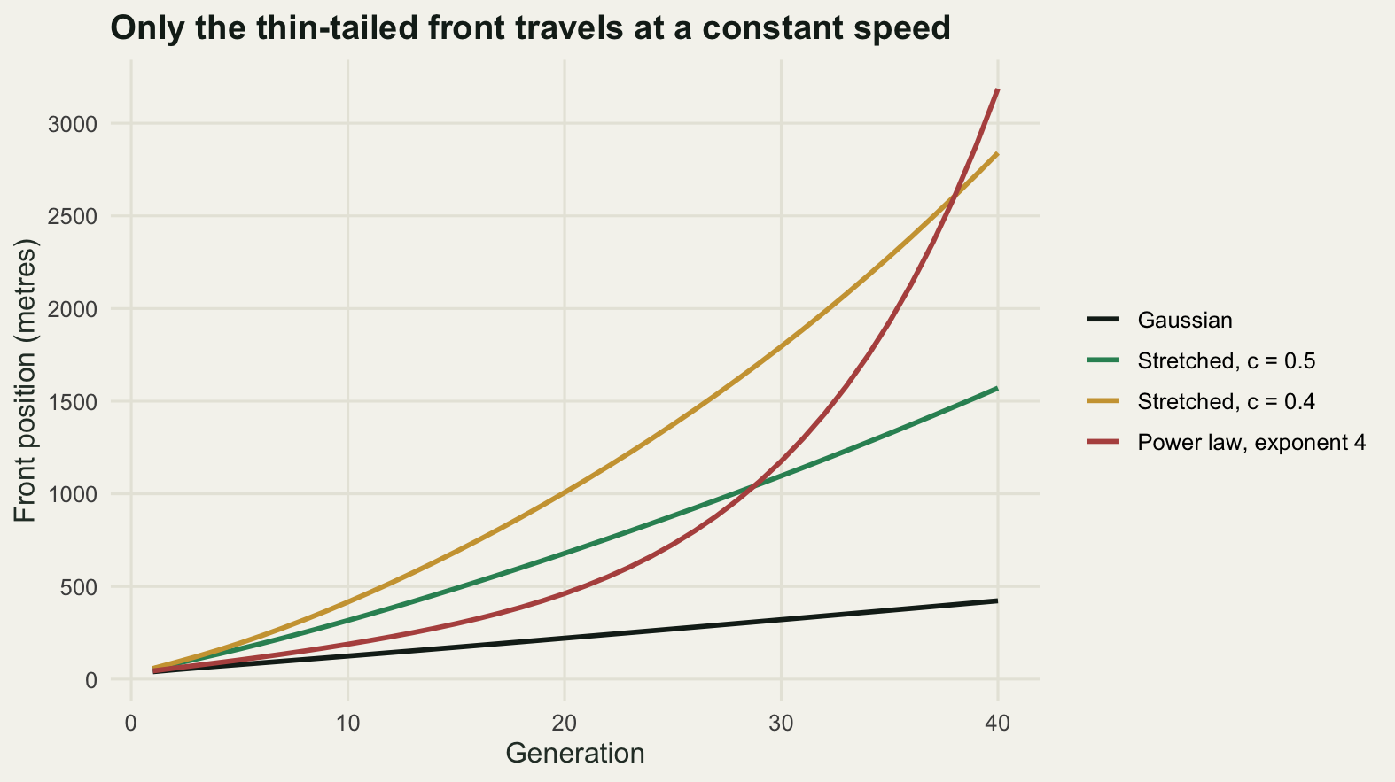

Figure 1: Front position against generation for four kernels that share a median jump of 8 metres and a growth rate of 1.5. The Gaussian trajectory is a straight line; the other three bend upwards, and the power law kernel, third of the four at generation 10, ends furthest ahead.

Fitting a power of time, and what it hides

The obvious way to summarise a superlinear trajectory is to fit a power of time, so regress the logarithm of front position on the logarithm of generation and read off the exponent. Because every run starts from an occupied patch 20 metres wide, the front position is measured from the edge of that patch rather than from the release point; otherwise the fitted exponent is pulled below one even for a perfectly straight line.

tt <- seq_len(tmax)
w1 <- tt >= 10
w2 <- tt >= 25
bfit <- function(y, ww) coef(lm(log(y[ww] - occupied) ~ log(tt[ww])))[[2]]
bb <- rbind(gen_10_to_40 = sapply(colnames(fr), function(nm) bfit(fr[, nm], w1)),
            gen_25_to_40 = sapply(colnames(fr), function(nm) bfit(fr[, nm], w2)))
print(round(bb, 3))

             gaussian   s50   s40 power
gen_10_to_40    0.979 1.197 1.419 2.137
gen_25_to_40    1.009 1.251 1.562 3.197

round(c(predicted_s50 = 1 / 0.5, predicted_s40 = 1 / 0.4), 3)

predicted_s50 predicted_s40 
          2.0           2.5 

Over generations 10 to 40 the exponents are 0.979 for the Gaussian, 1.197 and 1.419 for the two stretched exponentials, and 2.137 for the power law. The Gaussian result is the reassuring one: a front moving at constant speed has exponent one, and 0.979 is what a constant speed still converging upwards looks like. Over the later window, generations 25 to 40, it is 1.009.

The other three exponents are all larger than one, which settles the qualitative question, and all three drift upwards when the window is moved later, which is the warning. Asymptotic theory for a stretched exponential kernel with shape c says the front should grow like generation to the power 1 / c, that is 2 for shape 0.5 and 2.5 for shape 0.4. The measured 1.197 and 1.419 are nowhere near those. The fitted exponent is not converging to the theoretical one on any timescale a catchment partnership cares about.

Nothing is wrong with the theory; the log-log fit is the wrong instrument. For a stretched exponential the leading edge sits where the density, which is roughly the kernel tail multiplied by the compounded growth, crosses the threshold, and that condition reads as front position to the power c being linear in generation, not as front position being a power of generation. Those two statements differ by an additive constant inside a bracket, and an additive constant inside a bracket raised to a power of two or more takes an extremely long time to become negligible. The sharper test is therefore to raise the front position to the power c and regress that on generation directly, in which case the slope should be the logarithm of the growth rate.

sharp <- sapply(c("s50", "s40"), function(nm) {
  aa <- kl[[nm]]$par[["scale"]]
  cc <- kl[[nm]]$par[["shape"]]
  coef(lm(I((fr[w1, nm] / aa)^cc) ~ tt[w1]))[[2]]
})
round(c(sharp, target = log(growth), ratio_s50 = sharp[["s50"]] / log(growth),
        ratio_s40 = sharp[["s40"]] / log(growth)), 4)

      s50       s40    target ratio_s50 ratio_s40 
   0.4264    0.4007    0.4055    1.0517    0.9882 

pw <- c(gen_10_to_40 = coef(lm(log(fr[w1, "power"]) ~ tt[w1]))[[2]],
        gen_30_to_40 = coef(lm(log(fr[tt >= 30, "power"]) ~ tt[tt >= 30]))[[2]])
round(c(pw, target = log(growth) / 4,
        ratio_late = pw[["gen_30_to_40"]] / (log(growth) / 4)), 4)

gen_10_to_40 gen_30_to_40       target   ratio_late 
      0.0936       0.0997       0.1014       0.9836 

The slopes are 0.4264 and 0.4007 against a target of 0.4055, the logarithm of the growth rate: ratios of 1.0517 and 0.9882 against a target ratio of 1, on the same runs whose log-log exponents fell well short of the asymptotic value. The gap between shapes 0.5 and 0.4 is itself informative: the fatter kernel is closer to its asymptotic form at generation 40 because it gets there faster.

The power law kernel needs a different linearisation, and this is the part worth remembering. A polynomial tail with exponent 4 gives a front position whose logarithm is linear in generation, which is to say geometric growth of the distance itself. The predicted slope is the logarithm of the growth rate divided by the tail exponent, 0.1014. Measured over generations 10 to 40 it is 0.0936 and over generations 30 to 40 it is 0.0997, a ratio of 0.9836 to the prediction. A power-law tail does not merely make the front accelerate; it makes distance grow geometrically, so the front covers a fixed multiple of its current range in every fixed number of generations. That is why the power law starts third of four and finishes first.

fit_df <- do.call(rbind, lapply(colnames(fr), function(nm) {
  cf <- coef(lm(log(fr[w1, nm] - occupied) ~ log(tt[w1])))
  data.frame(gen = tt[w1], pos = exp(cf[[1]] + cf[[2]] * log(tt[w1])),
             kern = klab[[nm]])
}))
fit_df$kern <- factor(fit_df$kern, levels = klab)
ll_df <- front_df
ll_df$pos <- ll_df$pos - occupied

ggplot(ll_df[ll_df$gen >= 3, ], aes(gen, pos, colour = kern)) +
  geom_line(linewidth = 1) +
  geom_line(data = fit_df, linetype = "dashed", linewidth = 0.6,
            show.legend = FALSE) +
  scale_x_log10(breaks = c(3, 5, 10, 20, 40)) +
  scale_y_log10(breaks = c(30, 100, 300, 1000, 3000),
                labels = c("30", "100", "300", "1000", "3000")) +
  scale_colour_manual(values = setNames(as.character(kcol[names(klab)]), klab),
                      name = NULL) +
  labs(x = "Generation (log scale)", y = "Distance beyond the initial patch, metres",
       title = "A fitted power of time describes three of these four trajectories") +
  theme_te() +
  theme(legend.position = "right")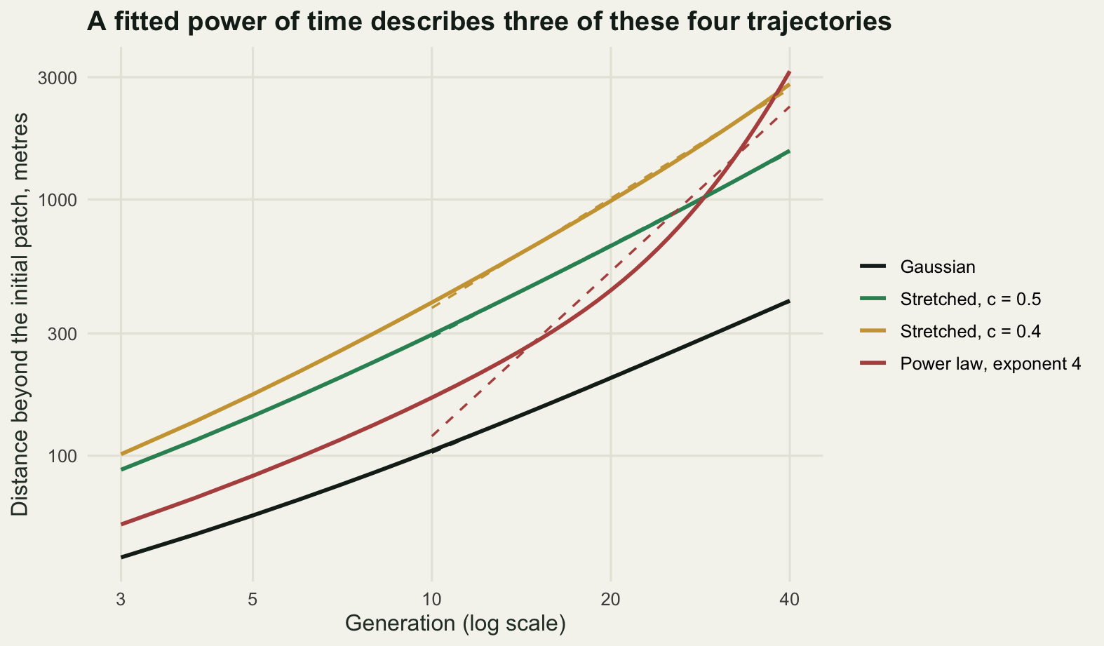

Figure 2: The same four trajectories on logarithmic axes, with dashed lines showing the power of generation fitted over generations 10 to 40. A constant speed is a straight line of slope one. The power law trajectory is not straight on these axes at all, because its distance grows geometrically rather than as a power of time.

The integral that decides whether a speed exists

Everything above is a symptom. The cause is a single integral. For a thin-tailed kernel the asymptotic front speed has a formula: pick a positive number s, multiply the growth rate by the moment generating function of the kernel evaluated at s, take the logarithm, divide by s, and minimise the result over s. The moment generating function is the average of the exponential of s times the displacement, and for a fat-tailed kernel that average does not exist. The exponential of a linear function outruns a tail that falls off more slowly than any exponential, so the integral diverges at every positive s. No integral, no minimum, no speed.

That is an analytic statement, and it can be watched happening. Sum the kernel weights multiplied by the exponential of s times the displacement, but only over displacements up to a cut-off, and then let the cut-off grow.

log_mgf <- function(kern, s, B, g = gr) {
  w <- cell_w(kern, g)
  keep <- abs(g$lg) <= B & w > 0
  z <- log(w[keep]) + s * g$lg[keep]
  mz <- max(z)
  (mz + log(sum(exp(z - mz)))) / log(10)
}

Bset <- c(50, 200, 1000, 5000)
mtab <- sapply(kl, function(k) sapply(Bset, function(B) log_mgf(k, 0.05, B)))
rownames(mtab) <- paste0("cutoff_", Bset, "m")
print(round(mtab, 3))

             gaussian    s50    s40  power
cutoff_50m      0.076  0.116  0.104  0.102
cutoff_200m     0.076  1.247  1.546  0.519
cutoff_1000m    0.076 13.911 15.681 14.640
cutoff_5000m    0.076 90.645 96.615 98.674

sset <- c(0.2, 0.1, 0.05, 0.02, 0.01)
mtab2 <- sapply(kl, function(k) sapply(sset, function(s) log_mgf(k, s, 16000)))
rownames(mtab2) <- paste0("s_", sset)
print(round(mtab2, 3))

       gaussian      s50      s40    power
s_0.2     1.223 1356.836 1369.844 1377.246
s_0.1     0.306  662.250  675.255  682.655
s_0.05    0.076  315.115  328.115  335.511
s_0.02    0.012  107.079  120.060  127.445
s_0.01    0.003   37.953   50.899   58.262

The table is on a base ten logarithmic scale because it has to be. At an s of 0.05 per metre the Gaussian sum is 0.076 whether the cut-off is 50 metres or 5000 metres: it converged before the first entry, and that number is the moment generating function. The other three start at much the same place, 0.116, 0.104 and 0.102 at a 50 metre cut-off, and then leave: by a 5000 metre cut-off they stand at 90.645, 96.615 and 98.674 on the same logarithmic scale. Nothing in that column is converging, and extending the cut-off further only makes the numbers larger. Lowering the value of s does not rescue it either. At an s of 0.01 per metre the Gaussian gives 0.003 while the three fat kernels give 37.953, 50.899 and 58.262 with the sum cut at 16 kilometres, and every one of those is still climbing with the cut-off.

The Gaussian case can be closed properly, which also calibrates the simulation against theory. For a Gaussian kernel the minimisation has a closed form: the asymptotic speed is the kernel standard deviation times the square root of twice the logarithm of the growth rate.

sg <- kl$gaussian$par[["scale"]]
cstar <- sg * sqrt(2 * log(growth))
cstar_num <- optimize(function(s) (log(growth) + log(10) * log_mgf(kl$gaussian, s, 16000)) / s,
                      c(1e-3, 0.5))$objective
zg <- run_ide(kl$gaussian, gr, growth, 120, thr_main)$pos[, 1]
sp_late <- coef(lm(zg[110:120] ~ I(110:120)))[[2]]
round(c(closed_form = cstar, from_grid_kernel = cstar_num,
        measured_gen_30_40 = coef(lm(fr[30:40, "gaussian"] ~ I(30:40)))[[2]],
        measured_gen_110_120 = sp_late, ratio = sp_late / cstar), 4)

         closed_form     from_grid_kernel   measured_gen_30_40 
             10.6809              10.6840              10.1771 
measured_gen_110_120                ratio 
             10.5272               0.9856 

The closed form gives 10.6809 metres a generation. Minimising numerically over the discrete grid kernel instead gives 10.684, so the discretisation is faithful. The simulated front moves at 10.1771 metres a generation over generations 30 to 40 and at 10.5272 over generations 110 to 120, which is 0.9856 of the predicted speed and still climbing. Pulled fronts approach their asymptotic speed from below and slowly, so the residual gap is expected rather than a failure of the model, and it is worth knowing that a run stopped at generation 40 still understates the thin-tailed speed: 10.1771 against the 10.6809 it is heading for. For the three fat kernels there is no such number to converge to.

s_show <- 0.05
pos_i <- which(gr$lg > 0 & gr$lg <= 4000 & gr$lg %% 2 == 0)
mg_df <- do.call(rbind, lapply(names(kl), function(nm) {
  w <- cell_w(kl[[nm]], gr)[pos_i]
  data.frame(dist = gr$lg[pos_i],
             contrib = log10(w) + s_show * gr$lg[pos_i] / log(10),
             kern = klab[[nm]])
}))
mg_df <- mg_df[is.finite(mg_df$contrib) & mg_df$contrib > -45, ]
mg_df$kern <- factor(mg_df$kern, levels = klab)

ggplot(mg_df, aes(dist, contrib, colour = kern)) +
  geom_hline(yintercept = 0, colour = te_pal$line, linewidth = 0.8) +
  geom_line(linewidth = 1) +
  scale_colour_manual(values = setNames(as.character(kcol[names(klab)]), klab),
                      name = NULL) +
  scale_x_log10(breaks = c(2, 10, 50, 200, 1000, 4000),
                labels = c("2", "10", "50", "200", "1000", "4000")) +
  coord_cartesian(ylim = c(-45, 60)) +
  labs(x = "Jump length (metres, log scale)",
       y = "Log base ten of the contribution",
       title = "A sum whose terms grow without bound is not a number") +
  theme_te() +
  theme(legend.position = "right")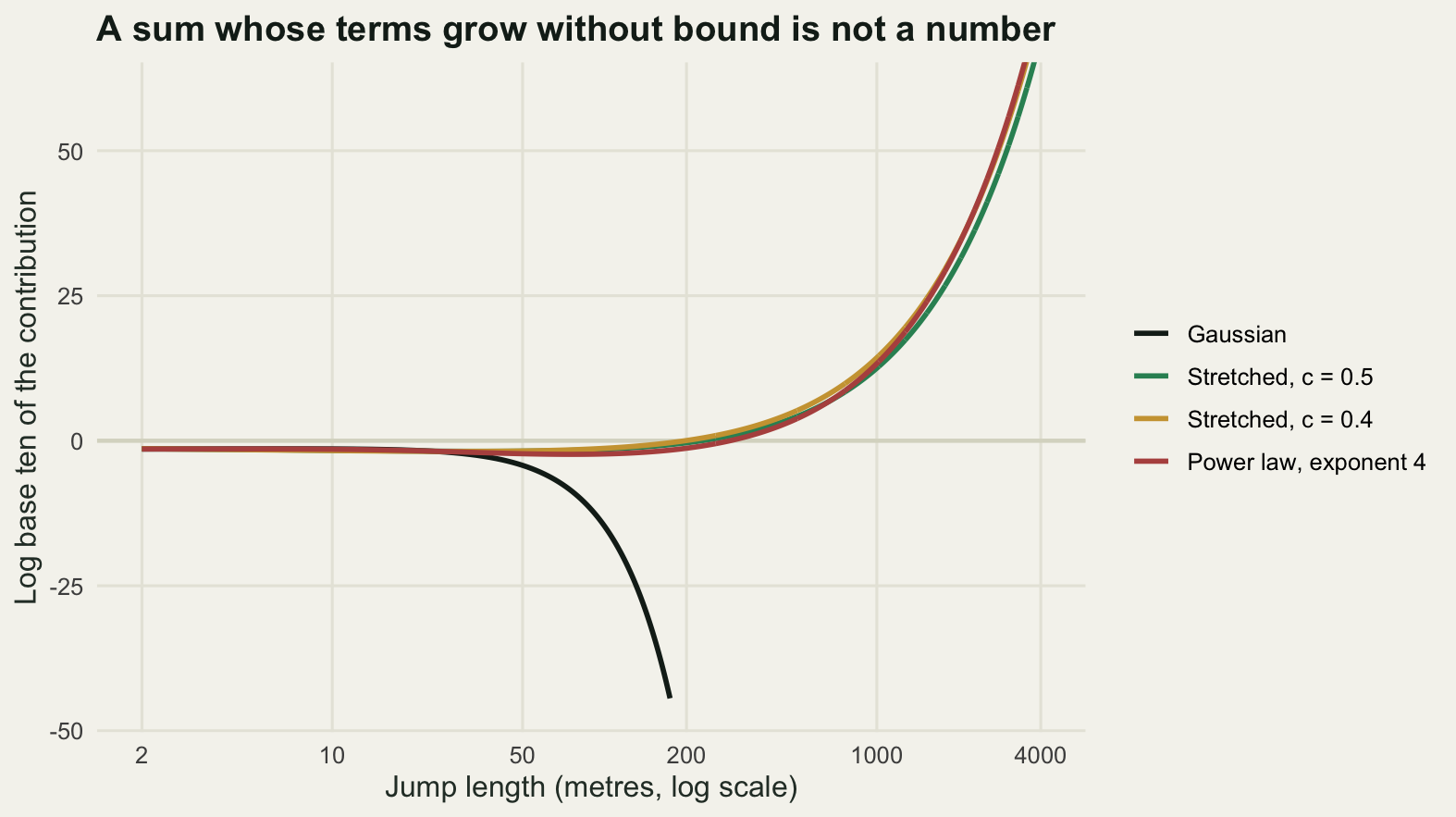

Figure 3: What each cell of the grid contributes to the moment generating function at an s of 0.05 per metre: the kernel weight for a jump of that length, multiplied by the exponential of s times the length. A sum converges only if its terms fall away to nothing. The Gaussian terms do, and leave the bottom of the panel before 200 metres. The other three turn round and climb.

A survey that cannot see the seeds that decide the answer

The comparison so far is between kernels chosen to be different. The uncomfortable case is the one in the field, where the kernel comes from data. Suppose the marked seed survey searched 60 metres up and down the corridor from the release point and recovered 400 seeds, and suppose the truth is a mixture: almost all seeds follow an exponential kernel with a median jump of 8 metres, while one seed in a thousand enters the water or is carried by an animal and follows a power-law kernel with a median jump of 200 metres.

r_max <- 60
n_seed <- 400
prop_true <- 0.001
med_far <- 200
nu_far <- 3
b_true <- med_jump / log(2)
s_far <- med_far / qt(0.75, nu_far)

G_far <- function(r) 2 * pt(r / s_far, nu_far) - 1
f_far <- function(r) 2 * dt(r / s_far, nu_far) / s_far
G_thin <- function(r, b) 1 - exp(-r / b)
f_thin <- function(r, b) exp(-r / b) / b
G_mix <- function(r, b, p) (1 - p) * G_thin(r, b) + p * G_far(r)

share <- prop_true * G_far(r_max) / G_mix(r_max, b_true, prop_true)
round(c(seeds = n_seed, search_radius_m = r_max, long_distance_fraction = prop_true,
        long_distance_median_m = med_far, far_share_of_recoveries = share,
        expected_far_seeds = n_seed * share), 6)

                  seeds         search_radius_m  long_distance_fraction 
             400.000000               60.000000                0.001000 
 long_distance_median_m far_share_of_recoveries      expected_far_seeds 
             200.000000                0.000168                0.067122 

set.seed(20260726)
rg <- seq(0, r_max, length.out = 200001)
rr <- approx(G_mix(rg, b_true, prop_true) / G_mix(r_max, b_true, prop_true), rg,
             xout = runif(n_seed))$y
round(c(n = length(rr), median_recovery = median(rr), max_recovery = max(rr)), 3)

              n median_recovery    max_recovery 
        400.000           8.032          58.010 

Within the search radius the long-distance component supplies 0.000168 of the recoveries: an expected 0.067 seeds out of 400. The survey has essentially no chance of catching one, and if it did catch one the seed would be indistinguishable from an ordinary recovery near the observed maximum of 58.010 metres. Fit the two models anyway, the pure exponential and the mixture, taking the shape of the long-distance component as known and its frequency as the one unknown.

nll <- function(b, p) -sum(log(((1 - p) * f_thin(rr, b) + p * f_far(rr)) /
                                 G_mix(r_max, b, p)))
prof <- function(p) optimize(function(lb) nll(exp(lb), p), c(-2, 6), tol = 1e-10)

p0 <- prof(0)
b_hat <- exp(p0$minimum)
pgrid <- c(0, exp(seq(log(1e-4), log(0.6), length.out = 60)))
devs <- sapply(pgrid, function(p) 2 * (prof(p)$objective - p0$objective))
p_up <- exp(uniroot(function(lp) 2 * (prof(exp(lp))$objective - p0$objective) - 3.841,
                    c(log(1e-4), log(0.6)))$root)

round(c(fitted_scale = b_hat, fitted_median = b_hat * log(2),
        aic_exponential = 2 * p0$objective + 2,
        aic_mixture = 2 * min(sapply(pgrid, function(p) prof(p)$objective)) + 4,
        min_deviance = min(devs), best_p = pgrid[which.min(devs)],
        upper_p = p_up, scale_at_upper_p = exp(prof(p_up)$minimum)), 4)

    fitted_scale    fitted_median  aic_exponential      aic_mixture 
         11.5061           7.9754        2729.1387        2731.1387 
    min_deviance           best_p          upper_p scale_at_upper_p 
          0.0000           0.0000           0.2896          10.4821 

The fitted exponential has a scale of 11.5061 metres, a median jump of 7.9754 metres, and an AIC of 2729.1387. The mixture is fitted best at a long-distance frequency of exactly zero, so its AIC is 2731.1387: worse by 2, which is the price of a parameter that bought nothing. On this survey the evidence for a long-distance component is not weak, it is absent, and an analyst reporting the model comparison honestly would report the exponential.

Now profile the likelihood in the other direction and ask what frequency of long-distance dispersal the survey rules out. The upper end of the 95 per cent likelihood interval for that frequency is 0.2896, against a truth of 0.001. The survey is consistent with that much long-distance dispersal because inside a 60 metre search radius a kernel with a 200 metre median looks almost flat, and the exponential scale simply shrinks from 11.5061 to 10.4821 metres to absorb it. Data censored at 60 metres carry no information about a process that operates at 200.

kern_mix <- function(m_thin, prop, m_far, nu) {
  bb <- m_thin / log(2)
  ss <- m_far / qt(0.75, nu)
  list(surv = function(r) (1 - prop) * exp(-r / bb) +
         prop * 2 * pt(r / ss, nu, lower.tail = FALSE),
       par = c(scale = bb, prop = prop))
}

kf <- list(fitted = kern_lap(b_hat * log(2)),
           truth = kern_mix(b_hat * log(2), prop_true, med_far, nu_far),
           allowed = kern_mix(b_hat * log(2), p_up, med_far, nu_far))
ff <- sapply(kf, function(k) run_ide(k, gr, growth, 30, thr_main)$pos[, 1])
rownames(ff) <- seq_len(30)
print(round(ff[c(10, 20, 30), ], 1))

   fitted  truth allowed
10  169.1  172.3  1498.1
20  311.4  709.9  4658.7
30  459.4 2262.6 11640.4

print(round(ff[c(10, 20, 30), ] / ff[c(10, 20, 30), "fitted"], 2))

   fitted truth allowed
10      1  1.02    8.86
20      1  2.28   14.96
30      1  4.93   25.34

long_thin <- run_ide(kf$fitted, gr, growth, 90, thr_main)$pos[, 1]
long_mid <- run_ide(kf$truth, gr, growth, 90, thr_main)$pos[, 1]
c(fitted = which(long_thin >= 1000)[1], truth = which(long_mid >= 1000)[1],
  allowed = unname(which(ff[, "allowed"] >= 1000)[1]))

 fitted   truth allowed 
     66      23       8 

mgf_lap <- function(s) 1 / (1 - (b_hat * s)^2)
round(c(thin_asymptotic_speed =
          optimize(function(s) (log(growth) + log(mgf_lap(s))) / s,
                   c(1e-4, 1 / b_hat - 1e-6))$objective,
        measured_gen_80_90 = coef(lm(long_thin[80:90] ~ I(80:90)))[[2]]), 4)

thin_asymptotic_speed    measured_gen_80_90 
              15.9439               15.5862 

Three kernels, all supported by the same 400 seeds, and three forecasts: the fitted exponential on its own, the same thin component with the true one in a thousand long jumps added, and the same again with the largest long-distance fraction the survey cannot reject. After 10 generations they give 169.1, 172.3 and 1498.1 metres. The first two stand in a ratio of 1.02, which is to say the first decade of monitoring cannot separate them either. After 20 generations they give 311.4, 709.9 and 4658.7 metres, a ratio of 2.28 between the first two. After 30 generations they give 459.4, 2262.6 and 11640.4 metres, a ratio of 4.93.

The fitted exponential kernel does have an asymptotic speed, and the run confirms it: 15.9439 metres a generation from the closed form, 15.5862 measured over generations 80 to 90. That is the seductive part. The number exists, it is stable, it can be quoted with a confidence interval, and it is an artefact of a family assumption the data never tested.

The management version is starker. Take a fixed line down the corridor, a kilometre from the release point, and ask when the front arrives. Under the fitted exponential kernel the answer is generation 66. Under the true mixture, in which one seed in a thousand travels a long way, it is generation 23. Under the frequency at the top of what the survey allows, it is generation 8. The exponential forecast is not slightly optimistic, and the survey it rests on cannot be blamed, because the survey was fitted correctly and the model comparison was done properly.

fc_lab <- c(fitted = "Fitted exponential kernel",
            truth = "Plus the true 1 in 1000 long jumps",
            allowed = "Plus the most the survey allows")
fc_df <- data.frame(gen = rep(seq_len(30), 3), pos = as.vector(ff),
                    model = factor(rep(fc_lab[colnames(ff)], each = 30),
                                   levels = fc_lab))

ggplot(fc_df, aes(gen, pos, colour = model)) +
  geom_hline(yintercept = 1000, linetype = "dashed", colour = te_pal$line,
             linewidth = 0.9) +
  geom_line(linewidth = 1) +
  annotate("text", x = 1.5, y = 1250, hjust = 0, size = 3.2, colour = "#2c3a31",
           label = "management boundary at 1 km") +
  scale_y_log10(breaks = c(30, 100, 300, 1000, 3000, 10000),
                labels = c("30", "100", "300", "1000", "3000", "10000")) +
  scale_colour_manual(values = c(te_pal$ink, te_pal$green, te_pal$clay), name = NULL) +
  labs(x = "Generation", y = "Front position, metres (log scale)",
       title = "The same 400 seeds support all three of these forecasts") +
  theme_te() +
  theme(legend.position = "right")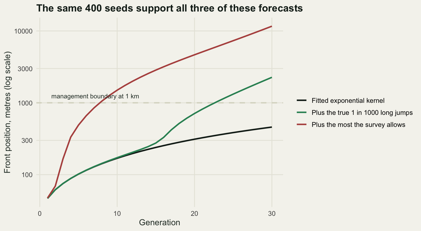

Figure 4: Three forecasts from one survey: the fitted exponential kernel on its own, the same kernel with the true one in a thousand long jumps added, and the same kernel with as many long jumps as the survey is unable to rule out. The dashed line marks a management boundary one kilometre down the corridor.

The honest limit

An accelerating front is a much less stable object to measure than a travelling wave, and three things about the measurements above deserve stating plainly.

The first is the definition of the front. For a thin-tailed kernel the asymptotic speed does not depend on the density threshold used to locate the leading edge; a different threshold shifts the line up or down without tilting it. That protection is gone here. The same runs measured at thresholds of 0.01 and 0.2 of carrying capacity give different exponents, because a fat-tailed front has no sharp edge to find: its profile ahead of the nominal front is a slowly decaying tail, not an exponential cliff.

The second is the grid. The kernel is truncated at the edge of the domain, so a domain that is too small silently deletes the long jumps that drive the whole phenomenon.

thr_tab <- t(sapply(names(res), function(nm) {
  z <- res[[nm]]$pos
  c(x40_thr_0.05 = z[40, 1], x40_thr_0.01 = z[40, 2], x40_thr_0.20 = z[40, 3],
    b_thr_0.05 = bfit(z[, 1], w1), b_thr_0.01 = bfit(z[, 2], w1),
    b_thr_0.20 = bfit(z[, 3], w1))
}))
print(round(thr_tab[, 1:3], 1))

         x40_thr_0.05 x40_thr_0.01 x40_thr_0.20
gaussian        422.8        449.9        391.9
s50            1570.8       1766.2       1393.2
s40            2839.8       3342.4       2414.1
power          3186.1       4804.0       2167.0

print(round(thr_tab[, 4:6], 3))

         b_thr_0.05 b_thr_0.01 b_thr_0.20
gaussian      0.979      0.896      1.111
s50           1.197      1.060      1.392
s40           1.419      1.273      1.629
power         2.137      2.200      2.095

coarse <- sapply(kl, function(k)
  run_ide(k, make_grid(2, 32768L), growth, 40, thr_main)$pos[40, 1])
print(round(rbind(fine_1m = fr[40, ], coarse_2m = coarse,
                  percent_difference = 100 * (coarse / fr[40, ] - 1)), 3))

                   gaussian      s50      s40    power
fine_1m             422.818 1570.763 2839.783 3186.112
coarse_2m           423.672 1572.681 2844.497 3199.465
percent_difference    0.202    0.122    0.166    0.419

edge <- sapply(c(2048L, 4096L, 8192L), function(nn)
  run_ide(kl$power, make_grid(1, nn), growth, 30, thr_main)$pos[30, 1])
round(c(half_width_2km = edge[1], half_width_4km = edge[2], half_width_8km = edge[3],
        half_width_16km = fr[30, "power"],
        percent_lost_at_2km = 100 * (edge[1] / fr[30, "power"] - 1)), 3)

     half_width_2km      half_width_4km      half_width_8km     half_width_16km 
            994.495            1176.227            1176.228            1176.228 
percent_lost_at_2km 
            -15.451 

cuts <- c(1e-13, 1e-10, 1e-8, 1e-5, 1e-3)
floor_tab <- t(sapply(cuts, function(fl)
  sapply(kl, function(k) run_ide(k, gr, growth, 40, thr_main, cut = fl)$pos[40, 1])))
rownames(floor_tab) <- paste0("cut_", format(cuts, scientific = TRUE))
print(round(floor_tab, 1))

          gaussian    s50    s40  power
cut_1e-13    422.8 1570.8 2839.8 3186.1
cut_1e-10    422.8 1570.3 2839.7 3186.1
cut_1e-08    422.8 1530.8 2657.3 2418.4
cut_1e-05    421.4 1358.5 2063.6  925.3
cut_1e-03    402.6 1083.3 1482.7  612.6

round(c(plants_per_metre_at_capacity = 400,
        metres_of_bank_per_plant_at_1e_8 = 1 / (400 * 1e-8)), 1)

    plants_per_metre_at_capacity metres_of_bank_per_plant_at_1e_8 
                             400                           250000 

Measured at a threshold of 0.01 instead of 0.05, the stretched exponential with shape 0.5 reaches 1766.2 metres instead of 1570.8 at generation 40, and its fitted exponent falls from 1.197 to 1.06; at a threshold of 0.2 it reaches 1393.2 metres with an exponent of 1.392. The power law spreads further still in position, 4804 metres against 2167 across the same two thresholds, though its exponent happens to be the most stable of the four. Any exponent quoted from a finite run is an exponent at a threshold, and it should be reported with one.

Halving the resolution to a two metre cell and doubling the domain changes the generation 40 front by at most 0.419 per cent, so the discretisation itself is not driving anything. Shrinking the domain does drive something: the power law front at generation 30 sits at 1176.2 metres on the 16 kilometre domain and on the 8 and 4 kilometre domains, but at 994.495 metres on a 2 kilometre domain, 15.45 per cent short, purely because jumps longer than 2 kilometres have been deleted from the kernel. A domain check is not optional in this kind of model, and the check has to be run at the horizon that will be reported, not at generation 10.

The third and largest limit is the one the deterministic model cannot fix. Setting all densities below a cut-off to zero each generation, which is what a population made of whole individuals does on its own, costs the fat-tailed fronts a great deal and the Gaussian front almost nothing. The first two rows of that table also settle the question left open earlier, which is what the numerical cut costs: moving it from 1e-13 to 1e-10 leaves every front unchanged at the tenth of a metre printed except the stretched exponential with shape 0.5, which slips from 1570.8 to 1570.3. Removing the round-off noise of the transform is free. Removing real individuals is not. At a cut-off of 1e-08 of carrying capacity the power law front falls from 3186.1 to 2418.4 metres; at 1e-05 it falls to 925.3; at 1e-03 it falls to 612.6, while the Gaussian front only drops from 422.8 to 402.6. If carrying capacity is 400 plants per metre of bank, a density of 1e-08 of capacity means one plant per 250000 metres of river. The accelerating front in the deterministic model is being pulled along by that, and it is a fiction: real spread at the leading edge is a matter of a handful of individuals arriving or not arriving, and the honest conclusion is that these trajectories are upper envelopes rather than predictions. What survives the criticism is the qualitative result, which does not depend on the fiction: a tail with no moment generating function has no speed to converge to, so a forecast made from it must be quoted as a range that widens with the horizon.

Where to go next

The rare long jump was treated here as one arm of a mixture in a deterministic model, which is the cheapest way to see what it does to the front. Treating it as a stochastic event that founds a new colony some distance ahead is more realistic and gives a different picture again, with the variance between replicates becoming the headline quantity rather than the mean: long-distance jumps and stratified spread does that. In the other direction, the mean dispersal distance is the statistic that goes infinite first when the tail gets fat, and it is worth knowing which of your summaries survive a power law and which do not.

Before either, it is worth running the checks in checking an invasion spread model on any spread model you intend to show anyone. The threshold sensitivity measured above is one of the four, and the other three are about how the front looks to a survey rather than how it behaves in a simulation.

References

Kot M, Lewis MA, van den Driessche P 1996 Ecology 77(7):2027-2042 (10.2307/2265698)

Clark JS 1998 American Naturalist 152(2):204-224 (10.1086/286162)

Nathan R 2006 Science 313(5788):786-788 (10.1126/science.1124975)

Kot M, Schaffer WM 1986 Mathematical Biosciences 80(1):109-136 (10.1016/0025-5564(86)90069-6)

Shigesada N, Kawasaki K 1997 Biological Invasions: Theory and Practice. Oxford University Press, ISBN 978-0-19-854851-5

Related tutorials

• Fat-tailed dispersal kernels
• The speed of an invasion front
• The mean dispersal distance
• Checking an invasion spread model