library(ggplot2)

te_pal <- list(forest = "#275139", green = "#2f8f63", sage = "#93a87f",
               clay = "#b5534e", gold = "#cda23f", line = "#dad9ca",
               ink = "#16241d", paper = "#f5f4ee")

theme_te <- function() {
  theme_minimal(base_size = 12) +
    theme(panel.grid.minor = element_blank(),
          panel.grid.major = element_line(colour = "#e7e6dc"),
          plot.background = element_rect(fill = "#f5f4ee", colour = NA),
          panel.background = element_rect(fill = "#f5f4ee", colour = NA),
          plot.title = element_text(face = "bold", colour = te_pal$ink),
          axis.title = element_text(colour = "#2c3a31"))
}Long-distance jumps and stratified spread
R
invasion ecology
dispersal
ecology tutorial
ggplot2
Rare long jumps found new foci ahead of an invasion front. Simulate stratified spread in R and measure the speed, the prediction variance and the payoff.
A pheromone trapping grid across a block of conifer plantations gives you one line on a map every autumn: the traps that caught something, and the traps that did not. Join up the outermost catches for five years running and the line creeps outwards at a steady couple of kilometres a year, which is the kind of number that goes into a briefing note and a spread model. Then a trap sixty kilometres beyond that line catches three males, and the site turns out to be a caravan park with a firewood pile.
That catch is not a wobble in the front position. It is a second spread process with its own rate and its own distance distribution, and it has just started a colony that will spread locally at the same couple of kilometres a year while producing outliers of its own. This tutorial builds the two processes on one grid and measures what the second one does: how much faster the invasion advances, how much less predictable its position becomes, where the switch from a front-dominated to a jump-dominated regime sits, and whether a fixed area of treatment buys more when it is spent at the front or on the outliers.
The four dispersal-kernel tutorials are the prerequisite here, not the competition: fitting dispersal kernels estimates a kernel from trap data, fat-tailed dispersal kernels measures how badly the tail is pinned down, and the mean dispersal distance shows what the tail does to a summary statistic. Turning a kernel into a speed is the job of the speed of an invasion front, and fat tails and accelerating spread does the same for a kernel with no finite moment generating function. This post keeps a thin-tailed local kernel, whose front therefore has a well behaved asymptotic speed, and adds a separate rare jump process on top of it. That is a modelling choice rather than a fact about the organism, and the last section says what it costs.
Two ways for the same population to move
The landscape is a one-dimensional transect of 1024 kilometres on a grid of half-kilometre cells, which is wide enough that nothing reaches either end within the horizon used here. Density is measured as a fraction of carrying capacity. Local spread is an integrodifference step: the population grows where it stands, then the offspring are redistributed by a Gaussian kernel with a standard deviation of two kilometres. Growth is Beverton-Holt with a low density multiplication rate of 1.8 a year, so a founding population multiplies while it is rare and flattens off as it fills the cell. A shared annual multiplier with a log standard deviation of 0.15 stands in for good and bad years, so two replicates with identical jumps still diverge slightly.
Convolution on a periodic grid is a multiplication in Fourier space, and base R has everything needed for it. mvfft transforms every replicate at once, which is what keeps a few hundred replicated runs inside a few seconds.
The mapped front is the furthest cell whose density reaches 0.05 of carrying capacity. That threshold is a survey design decision, not a property of the population, and the speed of an invasion front measures how little it matters for the asymptotic speed of a pulled front. It matters here for a different reason: a colony founded ahead of the front is invisible until it crosses the same threshold, and that delay turns out to be the largest single correction in the whole post.
dx <- 0.5; nx <- 2048L; i0 <- 201L
sigma_d <- 2; R0 <- 1.8; thr <- 0.05; env_sd <- 0.15
d_jump <- 12; found_peak <- 0.02; n_years <- 25L

make_kernel <- function(sig, ddx, nn) {
  kx <- (seq_len(nn) - 1) * ddx
  kx[kx > nn * ddx / 2] <- kx[kx > nn * ddx / 2] - nn * ddx
  k <- dnorm(kx, 0, sig) * ddx
  k / sum(k)
}
khat <- fft(make_kernel(sigma_d, dx, nx))
blob_h <- as.integer(ceiling(3 * sigma_d / dx))
blob <- found_peak * exp(-((-blob_h:blob_h) * dx)^2 / (2 * sigma_d^2))
blob_fast <- 3 * blob
cstar <- sigma_d * sqrt(2 * log(R0))

round(c(cell_km = dx, transect_km = nx * dx, kernel_sd_km = sigma_d,
        growth_rate = R0, map_threshold = thr, env_log_sd = env_sd,
        mean_jump_km = d_jump, founder_peak = found_peak,
        founder_mass_km = sum(blob) * dx, years = n_years,
        predicted_speed = cstar), 4)
cell_km transect_km kernel_sd_km growth_rate map_threshold
0.5000 1024.0000 2.0000 1.8000 0.0500
env_log_sd mean_jump_km founder_peak founder_mass_km years
0.1500 12.0000 0.0200 0.1001 25.0000
predicted_speed
2.1685 Two things in that block are worth pausing on. The founding colony is not a point: it is a Gaussian bump of peak density 0.02 and standard deviation two kilometres, holding as much population as 0.1001 kilometres of fully occupied transect. It is well below the mapping threshold when it lands. And the predicted speed, 2.1685 kilometres a year, comes from the standard linearised result for a thin-tailed kernel, which for a Gaussian reduces to the dispersal standard deviation times the square root of twice the log growth rate.
Before running anything stochastic, check that the deterministic engine reproduces that number, and check that the grid is not doing the work. The function below runs a jump-free deterministic front at three cell sizes and measures the speed over an early and a late window.
grid_speed <- function(ddx) {
  nn <- as.integer(1024 / ddx); ii <- as.integer(0.25 * nn) + 1L
  kh <- fft(make_kernel(sigma_d, ddx, nn))
  N <- numeric(nn); N[abs(seq_len(nn) - ii) * ddx <= 1] <- 1
  xs <- numeric(41)
  for (tt in 1:40) {
    G <- R0 * N / (1 + (R0 - 1) * N)
    N <- Re(fft(fft(G) * kh, inverse = TRUE)) / nn
    N[N < 0] <- 0
    xs[tt + 1] <- (max(which(N >= thr)) - ii) * ddx
  }
  c(years_5_to_25 = (xs[26] - xs[6]) / 20, years_20_to_40 = (xs[41] - xs[21]) / 20,
    edge_density = max(N[c(1:20, (nn - 19):nn)]))
}
gs <- sapply(c(1, 0.5, 0.25), grid_speed)
colnames(gs) <- c("dx_1_km", "dx_0.5_km", "dx_0.25_km")
print(round(gs, 4))
dx_1_km dx_0.5_km dx_0.25_km
years_5_to_25 2.0 2.0 2.000
years_20_to_40 2.1 2.1 2.075
edge_density 0.0 0.0 0.000round(c(predicted = cstar,
shortfall_percent_early = 100 * (1 - gs[1, "dx_0.5_km"] / cstar),
shortfall_percent_late = 100 * (1 - gs[2, "dx_0.5_km"] / cstar)), 4) predicted shortfall_percent_early shortfall_percent_late
2.1685 7.7694 3.1578 The measured speed over years 5 to 25 is 2.0 kilometres a year at all three cell sizes, and over years 20 to 40 it is 2.1 at the two coarser grids and 2.075 at the finest. Halving the cell twice leaves the early window unchanged and moves the late window only in its third significant figure, so the 7.77 per cent shortfall against the predicted 2.1685 is not a discretisation artefact. It is the finite-time approach of a pulled front to its asymptotic speed, which is slow and comes from below; the late window has closed a little under three fifths of the gap. Everything after this uses half-kilometre cells and a 25 year horizon, so the numbers are finite-time speeds, not asymptotic ones, and they sit a few per cent below the closed form on purpose.
The second calibration is the one that turns out to matter. Drop a founding colony on an empty transect and watch its peak density.
lag_run <- function(bl) {
  N <- numeric(nx); N[(i0 - blob_h):(i0 + blob_h)] <- bl
  pk <- numeric(13); pk[1] <- max(N)
  for (tt in 1:12) {
    G <- R0 * N / (1 + (R0 - 1) * N)
    N <- Re(fft(fft(G) * khat, inverse = TRUE)) / nx
    pk[tt + 1] <- max(N)
  }
  pk
}
pk <- lag_run(blob)
print(round(pk[1:8], 4))
[1] 0.0200 0.0251 0.0363 0.0552 0.0856 0.1327 0.2021 0.2973c(lag_years = which(pk >= thr)[1] - 1,
lag_years_dense_founder = which(lag_run(blob_fast) >= thr)[1] - 1) lag_years lag_years_dense_founder
3 0 The colony spends its first two years spreading faster than it grows, so its peak density climbs only from 0.02 to 0.0251 and then 0.0363, well short of the 1.8 a year the growth term on its own would give, and it only crosses the mapping threshold in year three, at 0.0552. Three years of invisibility does not sound like much. It costs more than half of the spread benefit of the jumps, as the sweep section measures.
What the jumps buy
The jump process is deliberately simple. In each year the number of successful foundings is Poisson with mean lambda, the founding site is drawn at an exponential distance with a mean of twelve kilometres beyond the current furthest mapped population, and each founding deposits the colony described above. Sourcing the jumps from the leading edge rather than from the whole occupied range is the assumption that makes this stratified diffusion rather than a fixed rain of outliers: a new colony, once mapped, becomes a source of further jumps.
All the random draws are generated in advance, so a managed run and its unmanaged baseline see exactly the same weather and exactly the same jumps. That pairing is what makes the management differences later on measurable with a few hundred replicates instead of a few thousand.
colcumsum <- function(m) {
  cs <- matrix(cumsum(m), nrow(m), ncol(m))
  cs - rep(c(0, cs[nrow(m), -ncol(m)]), each = nrow(m))
}

front_stats <- function(N) {
  ahead <- N[i0:nx, , drop = FALSE] >= thr
  nc <- nrow(ahead)
  imax <- i0 - 1L + apply(ahead * seq_len(nc), 2, max)
  cl <- colSums(colcumsum(1 - ahead) == 0)
  begins <- ahead & !rbind(rep(FALSE, ncol(ahead)), ahead[-nc, , drop = FALSE])
  list(imax = imax, xmax = (imax - i0) * dx, icont = i0 + cl - 1L,
       xcont = (cl - 1) * dx, nfoci = colSums(begins) - 1)
}

make_draws <- function(nrep, ny, lam, seed) {
  set.seed(seed)
  d <- list(Z = matrix(rnorm(ny * nrep), ny, nrep),
            NJ = matrix(rpois(ny * nrep, lam), ny, nrep), nrep = nrep, ny = ny)
  d$DJ <- lapply(seq_len(ny), function(tt) rexp(sum(d$NJ[tt, ]), 1 / d_jump))
  d
}

len_front <- 60; budget_km2 <- 120
front_cells <- as.integer(round(budget_km2 / len_front / dx))
man_start <- 6L; det_p <- 0.5
round(c(front_length_km = len_front, annual_budget_km2 = budget_km2,
        strip_depth_km = front_cells * dx, detection_probability = det_p,
        first_managed_year = man_start), 3)
front_length_km annual_budget_km2 strip_depth_km
60.0 120.0 2.0
detection_probability first_managed_year
0.5 6.0 run_sim <- function(dr, manage = "none", bl = blob, keep_field = FALSE, mseed = 4L) {
nrep <- dr$nrep; ny <- dr$ny
N <- matrix(0, nx, nrep); N[abs(seq_len(nx) - i0) * dx <= 1, ] <- 1
set.seed(mseed)
xmax <- matrix(0, ny + 1L, nrep); xcont <- xmax; nfoci <- xmax
fld <- if (keep_field) matrix(0, nx, ny + 1L) else NULL
if (keep_field) fld[, 1] <- N[, 1]
st <- front_stats(N); xmax[1, ] <- st$xmax; xcont[1, ] <- st$xcont
lost <- 0L; spent <- 0; jump_year <- numeric(0); jump_x <- numeric(0)
for (tt in seq_len(ny)) {
rr <- rep(R0 * exp(env_sd * dr$Z[tt, ]), each = nx)
G <- rr * N / (1 + (rr - 1) * N)
N <- Re(mvfft(mvfft(G) * khat, inverse = TRUE)) / nx
N[N < 0] <- 0
if (sum(dr$NJ[tt, ]) > 0) {
who <- rep(seq_len(nrep), dr$NJ[tt, ])
pos <- st$imax[who] + ceiling(dr$DJ[[tt]] / dx)
ok <- pos <= nx - blob_h
lost <- lost + sum(!ok)
for (q in which(ok)) {
w <- (pos[q] - blob_h):(pos[q] + blob_h)
N[w, who[q]] <- pmin(1, N[w, who[q]] + bl)
}
if (keep_field && any(who[ok] == 1L)) {
jump_year <- c(jump_year, rep(tt, sum(who[ok] == 1L)))
jump_x <- c(jump_x, (pos[ok][who[ok] == 1L] - i0) * dx)
}
}
st <- front_stats(N)
if (manage == "front" && tt >= man_start) {
rows <- outer(st$icont, 0:(front_cells - 1L), "-")
cols <- rep(seq_len(nrep), front_cells)
keep <- as.vector(rows) > i0
N[cbind(as.vector(rows)[keep], cols[keep])] <- 0
spent <- spent + sum(keep) * dx * len_front
st <- front_stats(N)
}
if (manage == "foci" && tt >= man_start) {
for (j in seq_len(nrep)) {
s0 <- st$icont[j] + 2L
if (s0 > nx) next
oc <- N[s0:nx, j] >= thr
if (!any(oc)) next
rl <- rle(oc)
ends <- cumsum(rl$lengths); begs <- ends - rl$lengths + 1L
sel <- which(rl$values)
sel <- sel[runif(length(sel)) < det_p]
if (!length(sel)) next
area <- pi * (rl$lengths[sel] * dx / 2)^2
o <- order(area)
take <- sel[o][cumsum(area[o]) <= budget_km2]
if (!length(take)) next
spent <- spent + sum(pi * (rl$lengths[take] * dx / 2)^2)
for (k in take) N[(s0 + begs[k] - 1L):(s0 + ends[k] - 1L), j] <- 0
}
st <- front_stats(N)
}
xmax[tt + 1L, ] <- st$xmax; xcont[tt + 1L, ] <- st$xcont
nfoci[tt + 1L, ] <- st$nfoci
if (keep_field) fld[, tt + 1L] <- N[, 1]
}
list(xmax = xmax, xcont = xcont, nfoci = nfoci, lost = lost, spent = spent,
edge = max(N[c(1:20, (nx - 19):nx), ]), field = fld,
jump_year = jump_year, jump_x = jump_x)
}Two runs of 250 replicates each, one with no jumps and one at half a successful founding a year, sharing their annual growth multipliers.
lam0 <- 0.5; nrep_main <- 250L
dA <- make_draws(nrep_main, n_years, 0, 11)
dB <- make_draws(nrep_main, n_years, lam0, 11); dB$Z <- dA$Z
A <- run_sim(dA); B <- run_sim(dB)
advA <- A$xmax[n_years + 1L, ]; advB <- B$xmax[n_years + 1L, ]
spA <- (advA - A$xmax[6, ]) / 20; spB <- (advB - B$xmax[6, ]) / 20

c(replicates = nrep_main, jump_rate = lam0)
replicates jump_rate
250.0 0.5 round(rbind(no_jumps = c(speed = mean(spA), speed_sd = sd(spA), advance = mean(advA),
advance_sd = sd(advA), cv = sd(advA) / mean(advA)),
with_jumps = c(mean(spB), sd(spB), mean(advB), sd(advB),
sd(advB) / mean(advB))), 4) speed speed_sd advance advance_sd cv
no_jumps 1.9970 0.0645 51.602 1.3044 0.0253
with_jumps 4.7684 1.2960 114.452 27.7517 0.2425round(c(speed_ratio = mean(spB) / mean(spA),
cv_ratio = (sd(advB) / mean(advB)) / (sd(advA) / mean(advA)),
jumps_per_replicate = mean(colSums(dB$NJ)),
coalesced_front_km = mean(B$xcont[n_years + 1L, ]),
foci_visible_at_25 = mean(B$nfoci[n_years + 1L, ]),
percent_with_a_visible_focus = 100 * mean(B$nfoci[n_years + 1L, ] >= 1),
percent_ever_showing_a_focus = 100 * mean(apply(B$nfoci, 2, max) >= 1),
prop_beyond_no_jump_maximum = mean(advB > max(advA))), 4) speed_ratio cv_ratio
2.3878 9.5924
jumps_per_replicate coalesced_front_km
12.5640 105.5140
foci_visible_at_25 percent_with_a_visible_focus
0.3000 28.0000
percent_ever_showing_a_focus prop_beyond_no_jump_maximum
91.6000 1.0000 round(c(no_jump_min = min(advA), no_jump_max = max(advA),
jump_q10 = quantile(advB, 0.1), jump_q90 = quantile(advB, 0.9),
jump_max = max(advB)), 2) no_jump_min no_jump_max jump_q10.10% jump_q90.90% jump_max
48.5 55.5 82.0 153.0 223.5 c(jumps_lost_off_the_grid = A$lost + B$lost)jumps_lost_off_the_grid
0 edge_max <- max(A$edge, B$edge)
signif(c(max_edge_density = edge_max), 3)max_edge_density
1.66e-10 Without jumps the front travels 51.602 kilometres in 25 years at 1.997 a year. With half a founding a year it travels 114.452 kilometres at 4.7684 a year, a factor of 2.3878 on the speed. The largest advance in 250 jump-free replicates is 55.5 kilometres, and every one of the 250 replicates with jumps finishes beyond it. That is what a rate of half an event a year does when each event is worth twelve kilometres and the local front is worth two.
The grid is not interfering: the highest density in the outermost twenty cells at either end is 1.66e-10, and no founding event landed off the transect.
The number that undercuts a common piece of field reasoning is the count of visible detached colonies. At year 25 the mean number of mapped patches ahead of the continuous invaded range is 0.3, and only 28 per cent of replicates show any at all, although 91.6 per cent showed one at some point during the run. The coalesced range edge stands at 105.514 kilometres against a furthest mapped population at 114.452. A single map of a stratified invasion mostly looks like a solid front, because the colonies that drive the advance are absorbed into the range within a few years of becoming visible. The absence of outliers on this year’s map says almost nothing about whether outliers are driving the spread.
ill_none <- run_sim(make_draws(1L, n_years, 0, 30), keep_field = TRUE)
ill_jump <- run_sim(make_draws(1L, n_years, lam0, 30), keep_field = TRUE)
c(illustrated_advance = ill_jump$xmax[n_years + 1L, 1],
  foundings_shown = length(ill_jump$jump_x), mean_advance = round(mean(advB), 2),
  pale_cutoff = 0.01)
illustrated_advance foundings_shown mean_advance pale_cutoff
113.50 12.00 114.45 0.01 cells <- seq(i0, i0 + 260L, by = 2L)
panel_of <- function(z, lab) {
m <- z$field[cells, ]
data.frame(x = rep((cells - i0) * dx, ncol(m)),
year = rep(0:n_years, each = length(cells)),
dens = as.vector(m), panel = lab)
}
lab_none <- "no jumps"; lab_jump <- "0.5 successful foundings a year"
sp_df <- rbind(panel_of(ill_none, lab_none), panel_of(ill_jump, lab_jump))
sp_df$panel <- factor(sp_df$panel, levels = c(lab_none, lab_jump))
sp_df$state <- ifelse(sp_df$dens >= thr, "mapped as present",
ifelse(sp_df$dens >= 0.01, "present, below the mapping threshold", NA))
sp_df <- sp_df[!is.na(sp_df$state), ]
jump_df <- data.frame(x = ill_jump$jump_x, year = ill_jump$jump_year,
panel = factor(lab_jump, levels = c(lab_none, lab_jump)))
ggplot(sp_df, aes(x, year, fill = state)) +
geom_tile(width = 1, height = 1) +
geom_point(data = jump_df, aes(x, year, shape = "founding event"),
inherit.aes = FALSE, colour = te_pal$clay, size = 2.2, stroke = 1) +
scale_shape_manual(values = c("founding event" = 4), name = NULL) +
facet_wrap(~panel) +
scale_y_reverse(breaks = seq(0, 25, by = 5)) +
scale_fill_manual(values = c("mapped as present" = te_pal$forest,
"present, below the mapping threshold" = te_pal$sage),
name = NULL) +
labs(x = "distance from the release point (km)", y = "year",
title = "The leading edge moves in steps, and the gap fills in behind it") +
theme_te() +
theme(legend.position = "top",
strip.text = element_text(colour = te_pal$ink, face = "bold"))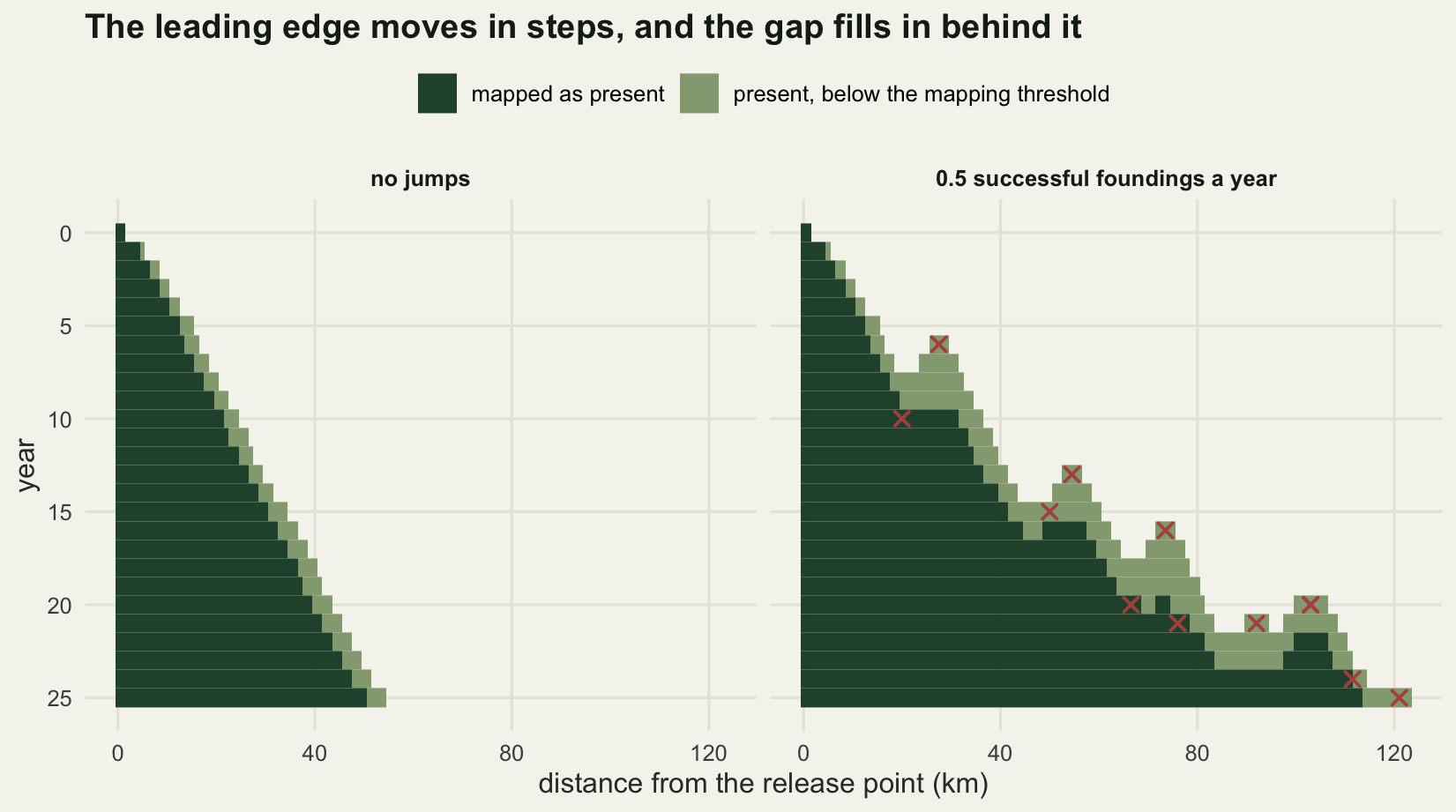
The variance is the finding
An invasion manager rarely needs the mean of a spread model. What is needed is a distance by which the thing will probably not have arrived, which is a quantile, and quantiles are where the two processes differ most.
round(c(no_jump_cv = sd(advA) / mean(advA), jump_cv = sd(advB) / mean(advB),
        no_jump_range_km = diff(range(advA)), jump_range_km = diff(range(advB)),
        no_jump_q90_minus_q10 = as.numeric(diff(quantile(advA, c(0.1, 0.9)))),
        jump_q90_minus_q10 = as.numeric(diff(quantile(advB, c(0.1, 0.9)))),
        jump_q95_km = as.numeric(quantile(advB, 0.95)),
        no_jump_q95_km = as.numeric(quantile(advA, 0.95))), 4)
no_jump_cv jump_cv no_jump_range_km
0.0253 0.2425 7.0000
jump_range_km no_jump_q90_minus_q10 jump_q90_minus_q10
164.0000 3.0000 71.0000
jump_q95_km no_jump_q95_km
163.2750 53.5000 The coefficient of variation of the 25 year advance is 0.0253 without jumps and 0.2425 with them, a factor of 9.5924. In kilometres, the tenth to ninetieth percentile range is 3.0 kilometres without jumps and 71.0 with them. A planner who wants a distance that will not be exceeded in nineteen runs out of twenty gets 53.5 kilometres from the jump-free model and 163.275 from the jump model, while the ratio of the mean speeds is only 2.3878. Nearly all of that extra spread comes from the jumps rather than from the weather: the annual growth multipliers are identical across the two runs.
band_of <- function(z, lab) {
  q <- apply(z$xmax, 1, quantile, probs = c(0.1, 0.9))
  data.frame(year = 0:n_years, mid = rowMeans(z$xmax), lo = q[1, ], hi = q[2, ],
             scenario = lab)
}
tr <- rbind(band_of(A, lab_none), band_of(B, lab_jump))
tr$scenario <- factor(tr$scenario, levels = c(lab_none, lab_jump))
show_id <- seq(1, nrep_main, length.out = 12)
ind <- data.frame(year = rep(0:n_years, length(show_id)),
                  x = as.vector(B$xmax[, show_id]),
                  id = rep(show_id, each = n_years + 1L))

ggplot(tr, aes(year, mid, colour = scenario, fill = scenario)) +
  geom_line(data = ind, aes(year, x, group = id), inherit.aes = FALSE,
            colour = te_pal$sage, linewidth = 0.35, alpha = 0.85) +
  geom_ribbon(aes(ymin = lo, ymax = hi), colour = NA, alpha = 0.3) +
  geom_line(linewidth = 1.1) +
  scale_colour_manual(values = c(te_pal$forest, te_pal$clay), name = NULL) +
  scale_fill_manual(values = c(te_pal$forest, te_pal$clay), name = NULL) +
  labs(x = "year", y = "distance of the furthest mapped population (km)",
       title = "Jumps lift the mean advance and stretch the spread around it") +
  theme_te() +
  theme(legend.position = "top")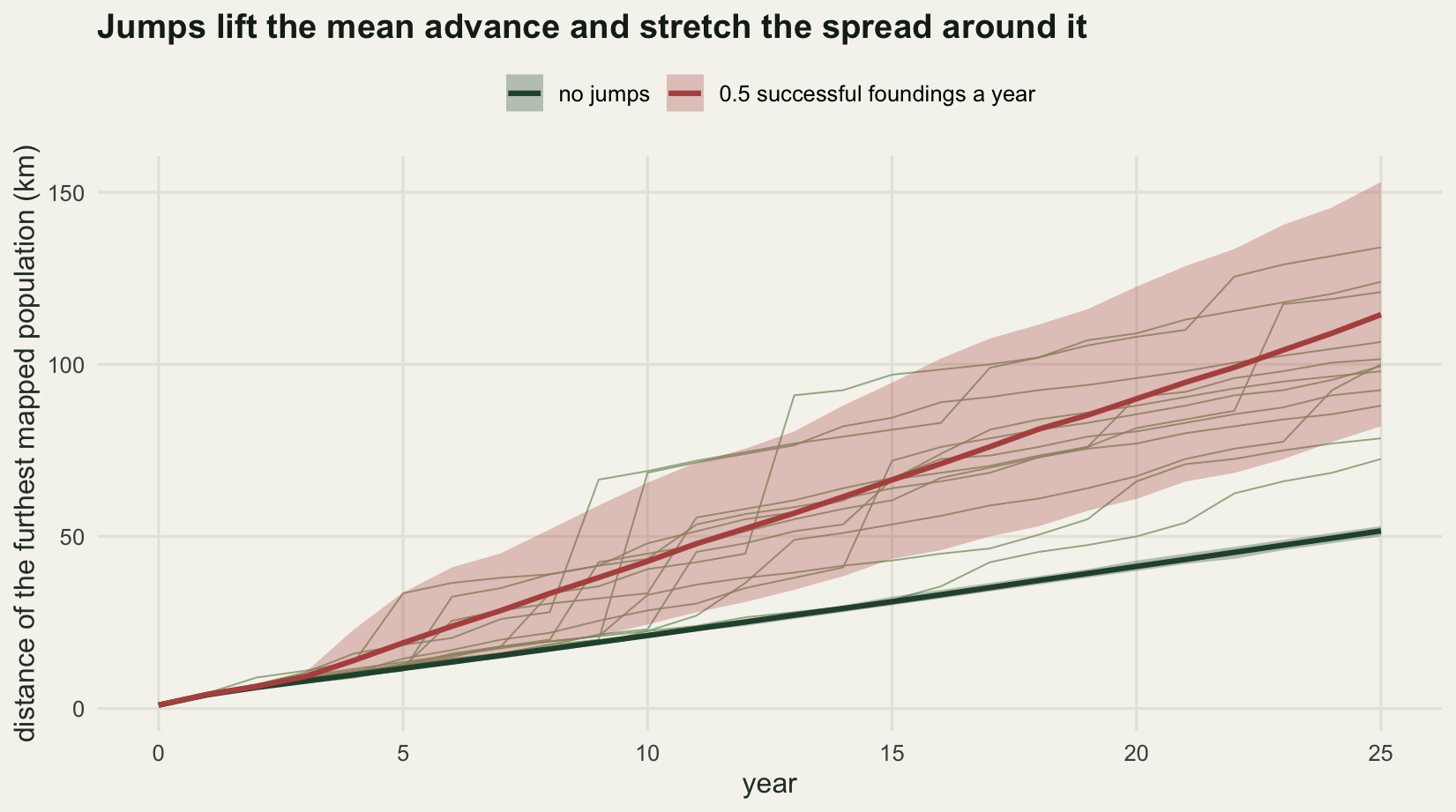
The individual replicate lines say more than the band does. Each one is a staircase: several years in which the leading edge creeps forward at the local rate, then a step of ten or twenty kilometres when a colony founded three years earlier crosses the mapping threshold. Fitting a straight line to one of those staircases, which is what a five year survey series amounts to, gives a slope that depends mostly on how many steps happened to fall inside the window.
Where the regime changes
Sweeping the founding rate from zero to 1.2 a year gives the shape of the transition. Two hundred replicates at each rate is enough for the mean advance; the coefficient of variation is noisier and its standard error is printed alongside.
lams <- c(0, 0.1, 0.2, 0.35, 0.5, 1.2)
nrep_s <- 200L
sw_runs <- lapply(seq_along(lams), function(i)
  run_sim(make_draws(nrep_s, n_years, lams[i], 100 + i)))
sw <- t(sapply(seq_along(lams), function(i) {
  adv <- sw_runs[[i]]$xmax[n_years + 1L, ]
  c(rate = lams[i], advance = mean(adv), advance_sd = sd(adv),
    cv = sd(adv) / mean(adv), cv_se = sd(adv) / mean(adv) / sqrt(2 * nrep_s),
    visible_foci = mean(sw_runs[[i]]$nfoci[n_years + 1L, ]),
    coalesced = mean(sw_runs[[i]]$xcont[n_years + 1L, ]))
}))
sw <- cbind(sw, jump_share = 1 - sw[1, "advance"] / sw[, "advance"])
print(round(sw, 4))
rate advance advance_sd cv cv_se visible_foci coalesced jump_share
[1,] 0.00 51.5950 1.3007 0.0252 0.0013 0.000 51.5950 0.0000
[2,] 0.10 68.5050 16.1991 0.2365 0.0118 0.065 66.1450 0.2468
[3,] 0.20 82.0725 22.5344 0.2746 0.0137 0.145 77.7125 0.3713
[4,] 0.35 98.8450 23.1400 0.2341 0.0117 0.195 93.4825 0.4780
[5,] 0.50 113.4825 29.8554 0.2631 0.0132 0.190 106.5900 0.5453
[6,] 1.20 163.8225 31.0724 0.1897 0.0095 0.435 150.8700 0.6851kk <- which(sw[, "jump_share"] >= 0.5)[1]
lam_star <- approx(sw[(kk - 1):kk, "jump_share"], lams[(kk - 1):kk], xout = 0.5)$y
fit <- lm(sw[, "advance"] ~ lams)
round(c(regime_threshold = lam_star, slope_km_per_year_per_unit_rate = coef(fit)[[2]] / 25,
intercept_km_per_year = coef(fit)[[1]] / 25, r_squared = summary(fit)$r.squared,
mean_jump_km = d_jump, share_of_mean_jump = coef(fit)[[2]] / 25 / d_jump), 4) regime_threshold slope_km_per_year_per_unit_rate
0.3990 3.5954
intercept_km_per_year r_squared
2.4473 0.9715
mean_jump_km share_of_mean_jump
12.0000 0.2996 c(replicates_each = nrep_s, jumps_lost_off_the_grid = sum(sapply(sw_runs, function(z) z$lost))) replicates_each jumps_lost_off_the_grid
200 0 Half of the 25 year advance is attributable to jumps once the founding rate passes 0.399 a year, and the sweep brackets that: at 0.35 the jump share is 0.478 and at 0.5 it is 0.5453. Below the threshold the local front is the invasion and the outliers are a nuisance; above it the front is mostly filling in ground that the outliers have already taken.
The mean advance is close to linear in the founding rate, with an r squared of 0.9715, which invites the obvious back of the envelope: each founding should add its expected distance of twelve kilometres, so the speed should rise by twelve kilometres a year for each extra founding a year. The measured slope is 3.5954, which is 0.2996 of that. The intercept, 2.4473 kilometres a year, sits about a fifth above the jump-free speed, because the advance climbs steeply between no foundings and 0.1 a year and the straight line has to lift its left-hand end to follow.
Two mechanisms take the missing seven tenths, and the first is bigger than I expected. A founding that lands in the last three years of the run never becomes visible, and every founding that lands while an earlier colony is still invisible is launched from a leading edge that is already out of date, so several jumps end up sharing one advance instead of adding to it. Rerunning the sweep with a founder dense enough to be mapped on arrival separates the two.
lams2 <- c(0, 0.35, 1.2)
sw2 <- t(sapply(seq_along(lams2), function(i) {
  z <- run_sim(make_draws(120L, n_years, lams2[i], 300 + i), bl = blob_fast)
  c(rate = lams2[i], replicates = 120, advance = mean(z$xmax[n_years + 1L, ]))
}))
print(round(sw2, 3))
rate replicates advance
[1,] 0.00 120 51.454
[2,] 0.35 120 139.225
[3,] 1.20 120 306.238fit2 <- lm(sw2[, "advance"] ~ lams2)
round(c(slope_no_lag = coef(fit2)[[2]] / 25, slope_with_lag = coef(fit)[[2]] / 25,
lost_to_the_lag = coef(fit2)[[2]] / 25 - coef(fit)[[2]] / 25,
share_of_mean_jump_no_lag = coef(fit2)[[2]] / 25 / d_jump), 4) slope_no_lag slope_with_lag lost_to_the_lag
8.3750 3.5954 4.7796
share_of_mean_jump_no_lag
0.6979 With the three year lag removed, the slope rises from 3.5954 to 8.375 kilometres a year per unit founding rate. The lag alone costs 4.7796 on this run, more than half of the gain the jumps would otherwise deliver. Even with no lag at all the slope reaches only 0.6979 of the mean jump distance, and that remaining shortfall is the overlap between jumps launched within the same short window from the same leading edge: what matters is the furthest of them, not their sum. The practical version of that sentence is that the frequency and the distance of long jumps do not enter a spread rate as a simple product, and a model that assumes they do will overpredict.
The coefficient of variation behaves differently again. It jumps from 0.0252 with no foundings to 0.2365 at a rate of 0.1 a year, sits between 0.2341 and 0.2746 across the middle of the sweep, where the differences are within about two standard errors of each other, and then falls to 0.1897 at 1.2 a year. The plateau and the decline are the law of large numbers arriving: at the top of the sweep a replicate collects enough foundings for the total distance jumped to start averaging out. Unpredictability is worst not where the jumps are commonest but where they are common enough to matter and rare enough to be counted on the fingers of one hand.
mlab <- c("mean advance in 25 years (km)", "share of the advance from jumps",
          "coefficient of variation")
sweep_df <- rbind(
  data.frame(rate = sw[, "rate"], y = sw[, "advance"], lo = NA, hi = NA, panel = mlab[1]),
  data.frame(rate = sw[, "rate"], y = sw[, "jump_share"], lo = NA, hi = NA, panel = mlab[2]),
  data.frame(rate = sw[, "rate"], y = sw[, "cv"], lo = sw[, "cv"] - 2 * sw[, "cv_se"],
             hi = sw[, "cv"] + 2 * sw[, "cv_se"], panel = mlab[3]))
sweep_df$panel <- factor(sweep_df$panel, levels = mlab)
fitline <- data.frame(rate = lams, y = fitted(fit), panel = factor(mlab[1], levels = mlab))
half <- data.frame(yint = 0.5, panel = factor(mlab[2], levels = mlab))
vline <- data.frame(xint = lam_star, panel = factor(mlab[2], levels = mlab))

ggplot(sweep_df, aes(rate, y)) +
  geom_hline(data = half, aes(yintercept = yint), colour = te_pal$line, linewidth = 0.9) +
  geom_vline(data = vline, aes(xintercept = xint), colour = te_pal$clay,
             linetype = "dashed", linewidth = 0.7) +
  geom_line(data = fitline, colour = te_pal$sage, linewidth = 0.9) +
  geom_errorbar(aes(ymin = lo, ymax = hi), width = 0.04, colour = te_pal$sage,
                na.rm = TRUE) +
  geom_line(colour = te_pal$forest, linewidth = 0.7) +
  geom_point(colour = te_pal$forest, size = 2.4) +
  facet_wrap(~panel, scales = "free_y") +
  labs(x = "successful foundings a year", y = NULL,
       title = paste0("Jumps take over the advance above about ",
                      round(lam_star, 2), " foundings a year")) +
  theme_te() +
  theme(strip.text = element_text(colour = te_pal$ink, face = "bold", size = 9))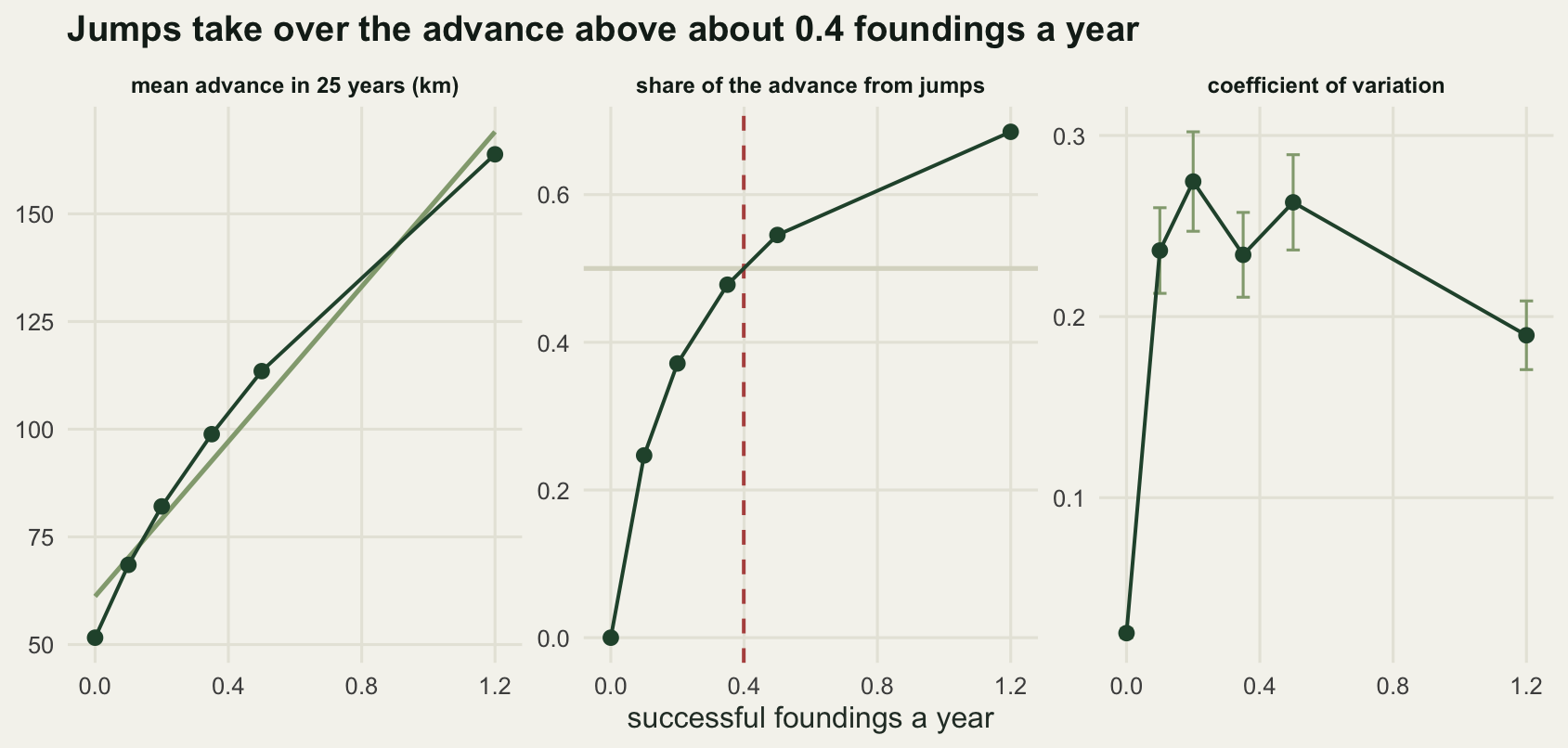
Two ways to spend the same area
Both management options are charged in treated area, which is the only currency in which they can honestly be compared. The invasion front is treated as a line 60 kilometres long across the landscape, so clearing a strip of depth two kilometres from the leading edge costs 120 square kilometres a year. A detached colony is treated as a circular patch, so eradicating one costs pi times the square of its radius, and colonies are treated cheapest first until the same annual 120 square kilometres is used up. Each visible colony is detected with probability 0.5 in each year, and both programmes start in year six. Nothing else differs: the managed runs reuse the sweep’s random draws, so each comparison is paired.
mi <- c(1, 3, 5, 6)
mg <- do.call(rbind, lapply(mi, function(i) {
  d <- make_draws(nrep_s, n_years, lams[i], 100 + i)
  base <- sw_runs[[i]]$xmax[n_years + 1L, ]
  o <- t(sapply(c("front", "foci"), function(s) {
    z <- run_sim(d, manage = s)
    dif <- base - z$xmax[n_years + 1L, ]
    c(advance = mean(z$xmax[n_years + 1L, ]), prevented = mean(dif),
      se = sd(dif) / sqrt(nrep_s), area = z$spent / nrep_s)
  }))
  data.frame(rate = lams[i], strategy = rownames(o), unmanaged = mean(base), o,
             row.names = NULL)
}))
mg$per_1000_km2 <- 1000 * mg$prevented / mg$area
mg$percent_prevented <- 100 * mg$prevented / mg$unmanaged
print(round(cbind(mg[, c("rate", "unmanaged", "advance", "prevented", "se", "area",
                         "per_1000_km2", "percent_prevented")]), 3))
rate unmanaged advance prevented se area per_1000_km2
1 0.0 51.595 46.127 5.468 0.096 2400.000 2.278
2 0.0 51.595 51.595 0.000 0.000 0.000 NaN
3 0.2 82.073 73.495 8.578 0.221 2400.000 3.574
4 0.2 82.073 78.622 3.450 0.601 27.198 126.846
5 0.5 113.482 104.265 9.217 0.300 2400.000 3.841
6 0.5 113.482 106.298 7.185 0.746 64.161 111.984
7 1.2 163.822 155.445 8.378 0.336 2400.000 3.491
8 1.2 163.822 149.395 14.428 1.101 90.573 159.291
percent_prevented
1 10.597
2 0.000
3 10.451
4 4.204
5 8.122
6 6.331
7 5.114
8 8.807print(mg$strategy)[1] "front" "foci" "front" "foci" "front" "foci" "front" "foci" dd <- mg$prevented[mg$strategy == "foci"] - mg$prevented[mg$strategy == "front"]
jj <- which(dd > 0)[1]
round(c(front_strip_km = front_cells * dx, cleared_depth_over_run_km =
front_cells * dx * (n_years - man_start + 1),
crossover_rate = approx(dd[(jj - 1):jj], lams[mi][(jj - 1):jj], xout = 0)$y,
foci_area_share_of_front_budget =
max(mg$area[mg$strategy == "foci"]) / mg$area[1]), 4) front_strip_km cleared_depth_over_run_km
2.0000 40.0000
crossover_rate foci_area_share_of_front_budget
0.6760 0.0377 Start with the jump-free case, because it sets the scale. The front programme clears the leading two kilometres of the invaded range every year from year six, which is 40 kilometres of clearance over the run against a front that advances about two kilometres a year. It prevents 5.468 kilometres of advance, with a paired standard error of 0.096. Clearing the leading edge of a pulled front is close to futile per unit of effort: the population immediately behind the cleared strip is at carrying capacity, and it refills most of the gap within the same year. The strip has to be cleared again next year, and the year after.
Prevention rises above 5.468 as soon as there are jumps, then stalls: the front programme prevents 8.578, 9.217 and 8.378 kilometres at founding rates of 0.2, 0.5 and 1.2. Because the total advance doubles across that range, its proportional benefit falls from 10.451 per cent to 5.114 per cent. The colony programme moves the other way, preventing nothing at all with no colonies to find, then 3.45, 7.185 and 14.428 kilometres. In absolute kilometres the two cross at a founding rate of 0.676, between the two rates that bracket it.
Per unit of area the comparison is not close at any rate above zero. The front programme spends 2400 square kilometres over the run and returns between 2.278 and 3.841 kilometres of prevented advance per thousand square kilometres treated. The colony programme spends at most 90.573 square kilometres, or 0.0377 of the same budget, and returns between 111.984 and 159.291 kilometres per thousand. The reason is geometric rather than ecological: a front is long and a colony is small, so a strip of front costs its length while a young colony costs the area of a circle a few kilometres across. That is the argument for nascent focus control, and here it is worth a factor of twenty or more. The NaN in the per_1000_km2 column at the zero founding rate is not a broken calculation: with no colonies to find, the colony programme treats no area and prevents no advance, so the ratio is zero divided by zero. The figure that follows plots it as a bar of height zero.
The colony programme never uses its budget, which is the second half of the result. It is limited by detection and by how quickly a colony outgrows what can be eradicated, not by treatment capacity. So the two are not really alternatives at all: a programme that finds and kills outliers leaves almost all of this budget unspent, and the sensible thing to do with the remainder is the front work that the per-area comparison has just made look pointless.
slab <- c(front = "clear the front", foci = "eradicate outlying colonies")
mplot <- rbind(
  data.frame(rate = factor(mg$rate), strategy = slab[mg$strategy], y = mg$prevented,
             lo = mg$prevented - mg$se, hi = mg$prevented + mg$se,
             panel = "advance prevented (km)"),
  data.frame(rate = factor(mg$rate), strategy = slab[mg$strategy],
             y = ifelse(is.finite(mg$per_1000_km2), mg$per_1000_km2, 0),
             lo = NA, hi = NA,
             panel = "prevented per 1000 square km treated (km)"))

ggplot(mplot, aes(rate, y, fill = strategy)) +
  geom_col(position = position_dodge(width = 0.75), width = 0.68) +
  geom_errorbar(aes(ymin = lo, ymax = hi), width = 0.16, colour = te_pal$ink,
                position = position_dodge(width = 0.75), na.rm = TRUE) +
  facet_wrap(~panel, scales = "free_y") +
  scale_fill_manual(values = c("clear the front" = te_pal$gold,
                               "eradicate outlying colonies" = te_pal$forest),
                    name = NULL) +
  labs(x = "successful foundings a year", y = NULL,
       title = "Front clearance prevents more kilometres only while jumps stay rare") +
  theme_te() +
  theme(legend.position = "top",
        strip.text = element_text(colour = te_pal$ink, face = "bold", size = 9))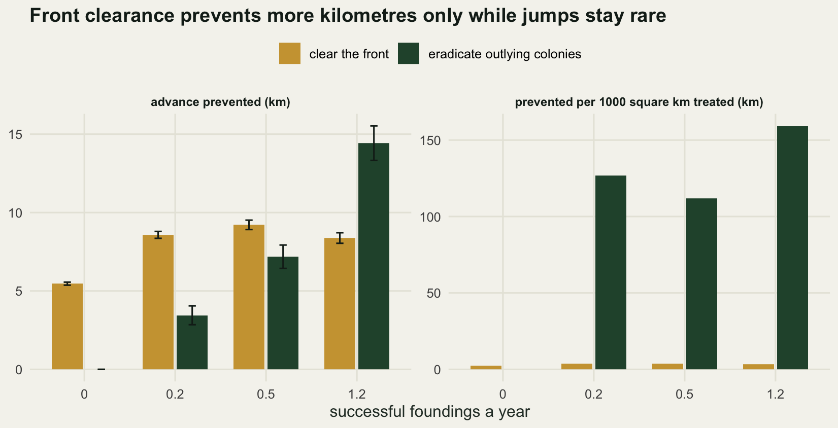
The honest limit
Every founding in this model succeeds. There is no Allee effect, no demographic stochasticity and no failure to find a mate, so a colony that lands is a colony that grows. The founding rate here is therefore the rate of successful establishments, not the rate of arrivals, and the two differ by a factor that is usually unknown and often very large. Allee effects and thresholds is where that factor lives, and it also removes the tidiest property used above: with a strong Allee effect a small founder can die out, so eradicating a colony and merely damaging it stop being the same thing.
The founding rate is also constant. In a real stratified invasion it grows with the invaded area, with the length of road inside it and with the volume of traffic leaving it, so the jump-driven component compounds rather than adding at a fixed rate. Everything measured above is therefore a lower bound on how far the jump process pulls ahead of the front over long horizons.
The management comparison rests on one number that was assumed rather than measured: the 60 kilometre front length that converts a strip depth into an area. Halve it and the same budget buys twice the strip depth; double it and the crossover at 0.676 moves down towards the founding rates at which programmes like this are actually run. The direction of the result is safe, because a front is long and a colony is compact in any real landscape, but that crossover rate is not transferable. Nor is search charged for: detection at 0.5 a year per visible colony is free in this model, and in the field it is the dominant cost of the outlier strategy and the reason programmes of this kind are usually built around volunteer reporting and trapping grids rather than systematic survey.
Finally, splitting dispersal into a Gaussian kernel plus a separate jump process is a modelling convenience. The same data could be described by one heavy-tailed kernel, and fat tails and accelerating spread shows what that alternative does to the front. The two descriptions are not equivalent: a heavy tail scales the jump distance with the amount of population at the source, while the process here fires at a fixed rate from the leading edge. Nothing in a seed trap or a pheromone grid will usually distinguish them, and they disagree about the far future.
Where to go next
The natural next step is to stop trusting the front position you measured. Checking an invasion spread model works through the failures that this post assumed away: what a detection lag does to an estimated speed, why a lag phase caused by slow establishment cannot be told from one caused by late detection, and how a strong Allee effect can stop a front outright and invalidate the linearised speed formula used at the top of this post.
If the outliers in your system are patches of habitat rather than points on a road, metapopulation capacity is the version of the same question for a fragmented landscape, where which patch is colonised next depends on the geometry of the network rather than on a single distance distribution.
References
Shigesada N, Kawasaki K, Takeda Y 1995 American Naturalist 146(2):229-251 (10.1086/285796)
Moody ME, Mack RN 1988 Journal of Applied Ecology 25(3):1009-1021 (10.2307/2403762)
Sharov AA, Liebhold AM 1998 Ecological Applications 8(3):833-845 (10.2307/2641270)
Liebhold AM, Tobin PC 2008 Annual Review of Entomology 53(1):387-408 (10.1146/annurev.ento.52.110405.091401)
Kot M, Lewis MA, van den Driessche P 1996 Ecology 77(7):2027-2042 (10.2307/2265698)