---
title: "Metapopulation capacity"
description: "Compute metapopulation capacity in R as the leading eigenvalue of the landscape matrix, rank patches by conservation value, and test the persistence threshold."
date: "2026-06-21 12:00"
date-modified: "2026-10-14"
categories: [R, metapopulation, spatial ecology, conservation, ecology tutorial]
image: thumbnail.png
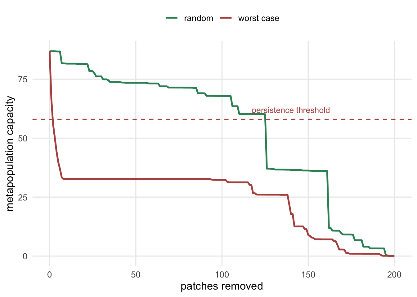
image-alt: "Two stepped curves of metapopulation capacity against the number of patches removed, both starting near 87 and ending at zero. The red curve collapses to about 33 within the first ten removals and then holds flat for a long stretch; the green curve slides gradually to about 60 by 120 removals, then falls in two big steps, to about 37 and then to about 11, before a short staircase takes it to zero. A dashed reference line sits near 58."
---
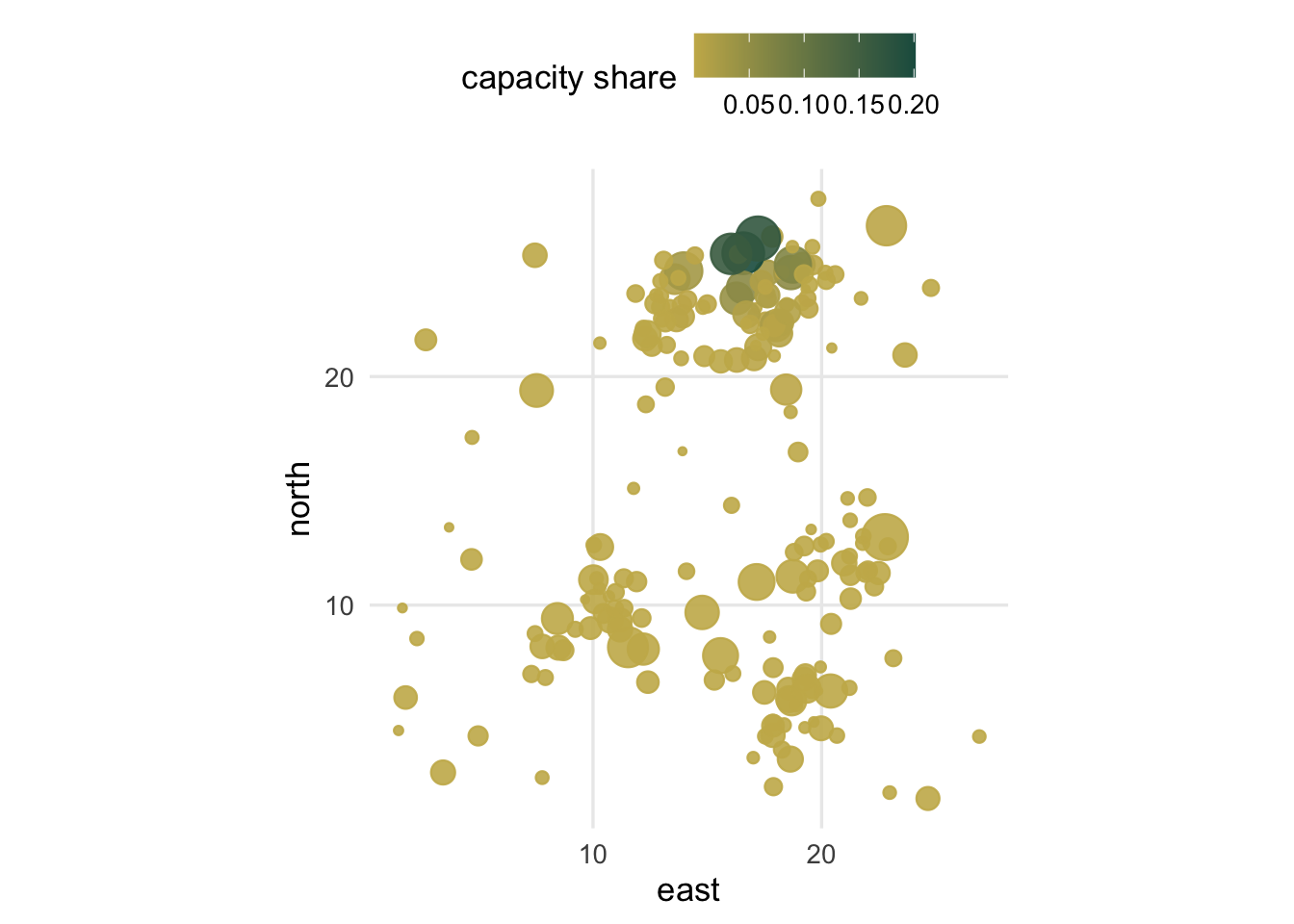
*Corrected 14 October 2026: the post called removing patches in the order of their single-patch value, ranked once in the intact landscape, the worst case, which it is not; it now calls it removal by value. The caption of the landscape map said that the large, well-connected patches carry the highest contributions and the small isolated ones little; it now says that the high contributions all sit in the dense northern group and that patches elsewhere, large ones included, contribute little.*
*Corrected 7 October 2026: the post gave the eigenvector approximation to the drop from removing a patch as twice the capacity times the squared eigenvector element, which overstates the exact drops about twofold; it now gives the capacity times the squared element. The share held by the five most valuable patches is now stated as a share of the summed single-patch drops, which exceed the capacity, rather than of an unnamed total.*
*Corrected 30 September 2026: the post reported one random removal order as what random loss does; it now says that this was a single, late-crossing draw and that other random orders cross the threshold much sooner.*
The Levins model gave a persistence rule for a soup of identical patches: the species holds on when its colonisation outpaces its extinction. Real landscapes are not a soup. Patches differ in size and sit at different distances, so the question becomes whether this particular arrangement of this particular set of patches can support the species. Ilkka Hanski and Otso Ovaskainen answered it in 2000 with a single number: the metapopulation capacity. It collapses the whole geometry of a patch network into one quantity that plays the role of the Levins threshold, and it comes with a bonus: it ranks every patch by how much it contributes to persistence. This post computes it in base R on the landscape from the incidence function tutorial, ranks the patches, and shows how fragile persistence can be when the best patches go first.
## From a rate to a landscape number
In the Levins world a species persists when a threshold is beaten. Hanski and Ovaskainen showed that once patches differ, the right generalisation of that threshold is an eigenvalue. Build a matrix `M` whose entry `M_ij` measures how strongly patch `j` can rescue or recolonise patch `i`: near patches with large areas exchange colonists readily, distant or tiny patches barely at all.
$$M_{ij} = e^{-\alpha\, d_{ij}}\, A_i A_j \quad (i \neq j), \qquad M_{ii} = 0.$$
The distance `d_ij` enters through the same dispersal kernel as before, and the areas `A_i A_j` weight the exchange by how much habitat sits at each end. The metapopulation capacity is the leading eigenvalue of this matrix, written `lambda_M`. A species with extinction-to-colonisation ratio `delta` persists in the landscape exactly when
$$\lambda_M > \delta.$$
The landscape supplies `lambda_M`; the species supplies `delta`. A demanding species (one that goes extinct easily or colonises weakly, so `delta` is large) needs a landscape with high capacity. The same landscape can hold a hardy species and lose a fragile one.
## Building the matrix
We use the clustered network from the incidence function tutorial: six clusters plus scattered isolates, 200 patches, a wide spread of areas, and the same dispersal parameter.
```{r}
#| label: landscape
set.seed(2024)
K <- 6; per <- 26
centres <- cbind(runif(K, 3, 25), runif(K, 3, 25))
clus <- do.call(rbind, lapply(1:K, function(k)
  cbind(rnorm(per, centres[k, 1], 1.3), rnorm(per, centres[k, 2], 1.3))))
iso <- cbind(runif(44, 1, 27), runif(44, 1, 27))
xy <- rbind(clus, iso)
n <- nrow(xy)
A <- rlnorm(n, meanlog = 0, sdlog = 0.9)
D <- as.matrix(dist(xy))
alpha <- 0.6
n
```
The capacity is one eigendecomposition away. The matrix is symmetric, so the eigenvector is real and, for a connected landscape, single-signed: every patch contributes to the leading mode.
```{r}
#| label: capacity
Mmat <- function(D, A, alpha) {
  M <- exp(-alpha * D) * outer(A, A)
  diag(M) <- 0
  M
}
M <- Mmat(D, A, alpha)
ev <- eigen(M, symmetric = TRUE)
lamM <- ev$values[1]
v <- abs(ev$vectors[, 1])
v <- v / sqrt(sum(v^2))
c(lambda_M = round(lamM, 2), eigenvector_single_signed = all(ev$vectors[, 1] > 0) || all(ev$vectors[, 1] < 0))
```
This landscape has a capacity of `r round(lamM,1)`. On its own that number means nothing; it becomes a verdict only against a species `delta`. Suppose a species with `delta` = 58. The rule asks whether the capacity clears that threshold, and the next sections take patches out of the landscape and watch the comparison move.
```{r}
#| label: fig-landscape
#| fig-cap: "The patch network, each patch sized by area and shaded by its contribution to metapopulation capacity. The highest contributions all sit in the dense northern group, led by a few large patches there; patches elsewhere, large ones included, contribute little."
#| fig-alt: "A square landscape of circles in dense groups and loose singletons. A few large circles are shaded dark green (high contribution); most circles are small and pale yellow (low contribution)."
#| echo: false
#| warning: false
library(ggplot2)
te_canvas <- theme(plot.background = element_rect(fill = "#f5f4ee", colour = NA),
panel.background = element_rect(fill = "#f5f4ee", colour = NA))
dfl <- data.frame(x = xy[, 1], y = xy[, 2], area = A, contrib = v^2)
ggplot(dfl, aes(x, y, size = area, colour = contrib)) +
geom_point(alpha = 0.9) +
scale_size_area(max_size = 8, guide = "none") +
scale_colour_gradient(low = "#c9b458", high = "#1d5b4e", name = "capacity share",
breaks = c(0.05, 0.15),
guide = guide_colourbar(barwidth = grid::unit(6, "cm"),
barheight = grid::unit(0.35, "cm"))) +
coord_equal() +
labs(x = "east", y = "north") +
theme_minimal(base_size = 13) + te_canvas +
theme(panel.grid.minor = element_blank(), legend.position = "top")
```
## Which patches matter
The capacity ranks patches for free. The value of a patch is how much capacity the landscape loses when that patch is destroyed: delete row and column `i` from `M`, recompute the leading eigenvalue, and take the drop. Do it for all 200.
```{r}
#| label: patch-value
drop <- sapply(1:n, function(i)
  lamM - eigen(M[-i, -i], symmetric = TRUE, only.values = TRUE)$values[1])
ord <- order(drop, decreasing = TRUE)
top5 <- round(drop[ord[1:5]], 2)
share5 <- 100 * sum(drop[ord[1:5]]) / sum(drop)
trivial <- sum(drop < 0.01 * lamM)
list(top5_values = top5, top5_share_pct = round(share5, 1), patches_under_1pct = trivial)
```
The five most valuable patches account for `r round(share5,0)`% of the summed single-patch drops, and `r trivial` of the `r n` patches each contribute less than one per cent of the capacity. The single most valuable patch is number `r ord[1]`, with area `r round(A[ord[1]],2)`; removing it alone drops the capacity from `r round(lamM,1)` to `r round(lamM-drop[ord[1]],1)`, a loss of `r round(100*drop[ord[1]]/lamM,0)`%.
You do not actually need 200 eigendecompositions to find these patches. Hanski and Ovaskainen showed that a patch's contribution is close to the square of its leading eigenvector element; the drop from removing patch `i` is well approximated by `lambda_M * v_i^2`.
```{r}
#| label: approx
approx <- lamM * v^2
c(correlation = round(cor(drop, approx), 4),
  rank_correlation = round(cor(drop, approx, method = "spearman"), 4))
```
The eigenvector approximation tracks the exact removal drop with a correlation of `r round(cor(drop,approx),3)` and a rank correlation of `r round(cor(drop,approx,method='spearman'),5)`, both printed to four decimals in the block above. So the leading eigenvector is a ready-made map of conservation priority: patches with large `v_i` are the ones to protect.
## Fragility: when the best patches go first
Habitat loss rarely falls evenly. If development or degradation takes the highest-value patches first, the capacity falls faster than the patch count suggests. Compare two removal orders: by value (remove patches in the order of their single-patch value, ranked once in the intact landscape) against neutral (remove them at random).
```{r}
#| label: removal
delta <- 58
lam_seq <- numeric(n + 1); lam_seq[1] <- lamM; keep <- rep(TRUE, n)
for (k in 1:n) {
  keep[ord[k]] <- FALSE
  lam_seq[k + 1] <- if (sum(keep) >= 2)
    eigen(M[keep, keep], symmetric = TRUE, only.values = TRUE)$values[1] else 0
}
set.seed(11)
lam_rnd <- numeric(n + 1); lam_rnd[1] <- lamM; keepr <- rep(TRUE, n); rnd <- sample(n)
for (k in 1:n) {
  keepr[rnd[k]] <- FALSE
  lam_rnd[k + 1] <- if (sum(keepr) >= 2)
    eigen(M[keepr, keepr], symmetric = TRUE, only.values = TRUE)$values[1] else 0
}
cross_val <- which(lam_seq < delta)[1] - 1
cross_rnd <- which(lam_rnd < delta)[1] - 1
c(by_value = cross_val, at_random = cross_rnd)
```
Removing the most valuable patches first, the capacity is below the species threshold once `r cross_val` of `r n` patches have gone; the first three removals take it from `r round(lamM,1)` to `r round(lam_seq[2],1)`, `r round(lam_seq[3],1)`, then `r round(lam_seq[4],1)`. Removing patches in one random order, the same landscape is below the threshold after `r cross_rnd`. That is a single draw, and a late one: other random orders cross the threshold at very different points, most of them much sooner, so a fair comparison uses the spread over many random orders. Even against that spread, value-ordered loss crosses far sooner than typical random loss. The capacity depends on which patches remain, not only on how many, so a count of habitat lost says little on its own.
```{r}
#| label: fig-removal
#| fig-cap: "Metapopulation capacity as patches are removed, by value (highest single-patch value first, ranked once in the intact landscape) against random order. The dashed line is the species persistence threshold."
#| fig-alt: "Two declining curves of capacity against number of patches removed. The by-value curve plunges steeply and crosses a dashed horizontal threshold near the left; the random curve declines gently and crosses it much further right."
#| echo: false
#| warning: false
dfr <- data.frame(
removed = rep(0:n, 2),
lambda = c(lam_seq, lam_rnd),
order = rep(c("by value", "random"), each = n + 1))
ggplot(dfr, aes(removed, lambda, colour = order)) +
geom_hline(yintercept = delta, linetype = "dashed", colour = "#b5534e") +
geom_line(linewidth = 1) +
annotate("text", x = n * 0.7, y = delta + 4, label = "persistence threshold",
colour = "#b5534e", size = 3.5) +
scale_colour_manual(values = c("by value" = "#b5534e", "random" = "#2f8f63"), name = NULL) +
labs(x = "patches removed", y = "metapopulation capacity") +
theme_minimal(base_size = 13) + te_canvas +
theme(panel.grid.minor = element_blank(), legend.position = "top")
```
## The honest limit: it all rides on the kernel
The capacity is only as trustworthy as the dispersal parameter fed into it. That parameter, `alpha`, is the one the incidence function tutorial fixed by hand because a snapshot cannot pin it down, and the capacity is sensitive to it. Recompute `lambda_M` across a range.
```{r}
#| label: alpha-sens
lamOf <- function(a) eigen(Mmat(D, A, a), symmetric = TRUE, only.values = TRUE)$values[1]
als <- c(0.3, 0.6, 1.0, 1.5)
lams <- sapply(als, lamOf)
persists <- lams > delta
data.frame(alpha = als, lambda_M = round(lams, 1), persists = persists)
```
As `alpha` moves from 0.3 to 1.5, the capacity slides from `r round(lamOf(0.3),0)` down to `r round(lamOf(1.5),0)`. Against `delta` = 58 the verdict can flip within that range: a small `alpha` is a shallow decay, so the same map can support the species under a long-distance kernel and not under a short-distance one. The reassuring part, which the table above does not show, is that the ranking of patches is far steadier than the verdict: the top few patches stay near the top across kernels, so a conservation priority list is less sensitive to getting `alpha` wrong than a yes-or-no persistence call is. Still, any absolute claim from `lambda_M` inherits the uncertainty in `alpha`, which is exactly why the checking tutorial insists that parameter be reported with its full width, not as a point.
That coupling is the theme of the last tutorial in this set: the persistence threshold is a clean line in theory, but every ingredient that feeds it (the kernel, the equilibrium assumption, the finiteness of a real population) blurs it. A number as tidy as `lambda_M` earns its keep only alongside the checks that say how much to trust it.
## References
Hanski I, Ovaskainen O 2000 Nature 404(6779):755-758 (10.1038/35008063)
Ovaskainen O, Hanski I 2001 Theoretical Population Biology 60(4):281-302 (10.1006/tpbi.2001.1548)
Hanski I 1999 Metapopulation Ecology, Oxford University Press, ISBN 978-0-19-854065-6
Hanski I, Gilpin M 1991 Biological Journal of the Linnean Society 42(1-2):3-16 (10.1111/j.1095-8312.1991.tb00548.x)
Ovaskainen O, Hanski I 2003 Theoretical Population Biology 64(4):481-495 (10.1016/S0040-5809(03)00102-3)
## Related tutorials
- [The Levins metapopulation model](../the-levins-metapopulation-model/)
- [The incidence function model](../incidence-function-model/)
- [Checking a metapopulation model](../checking-a-metapopulation-model/)
- [Long-distance jumps and stratified spread](../stratified-diffusion-and-long-distance-jumps/)