---
title: "The incidence function model"
description: "Fit Hanski's incidence function model to one snapshot of patch occupancy in R: patch area drives extinction, connectivity drives colonisation of empty patches."
date: "2026-06-21 11:00"
date-modified: "2026-10-14"
categories: [R, metapopulation, spatial ecology, imperfect detection, ecology tutorial]
image: thumbnail.png
image-alt: "A map of habitat patches drawn as circles sized by area, some filled dark green and some left open. The filled circles gather into a few dense clumps, while the open ones sit both inside those clumps and scattered thinly across the emptier parts of the map. Faint grey gridlines are the only other marks."
---
*Corrected 14 October 2026: the profile intervals were read off the grid points inside the cut-off, which made each one slightly too narrow; each end is now found where the profile crosses the cut-off between two grid points, and the other two parameters are refitted from several starts at each point.*
*Corrected 1 October 2026: the area-only fit in the connectivity test started from a single point and stopped at a lower local maximum of its likelihood, which overstated the gain from adding connectivity; it is now fitted from several starts, and the reported deviance is smaller and the p-value larger, with the same conclusion. The screen-reader description of the fitted-incidence figure also said incidence rises from low values at small areas; it now describes the flat band just below one half there.*
The Levins model treats every patch as identical and equally reachable. Real fragmented landscapes are not like that: a large patch holds a population more securely than a small one, and a colonist is far more likely to land on a nearby patch than a distant one. Ilkka Hanski's incidence function model, published in 1994, keeps the colonisation-extinction logic of Levins but lets patch area set the extinction risk and lets connectivity set the colonisation chance. Its selling point is practical: it can be fitted to a single snapshot of which patches are occupied, without watching the network through time. This post builds the model in base R, fits it to a simulated snapshot, and shows both what it recovers and what it leans on to do so.
## The model, patch by patch
Each patch `i` has an area `A_i` and a location. Two functions govern its fate.
Extinction of an occupied patch falls with area:
$$E_i = \min\!\left(1,\ \frac{\mu}{A_i^{\,x}}\right).$$
Large patches are hard to lose (small `E_i`); tiny patches blink out readily. The exponent `x` sets how steeply extinction drops with area.
Colonisation of an empty patch rises with connectivity. Connectivity `S_i` sums the contributions of every occupied patch, each weighted by its area and discounted by distance through a dispersal kernel with parameter `alpha`:
$$S_i = \sum_{j \neq i} o_j\, e^{-\alpha\, d_{ij}}\, A_j, \qquad C_i = \frac{S_i^2}{S_i^2 + y^2}.$$
Here `o_j` is one if patch `j` is occupied. A well-connected patch (many large occupied neighbours nearby) has a high `C_i`; an isolated one has a low `C_i`. The scaling `y` sets the connectivity at which colonisation reaches one half.
Now the trick that makes a snapshot enough. A patch behaves as a two-state chain: when empty it fills with probability `C_i`, when occupied it empties with probability `E_i`. The long-run probability that such a patch is occupied, its incidence, is
$$J_i = \frac{C_i}{C_i + E_i}.$$
If the network sits at its stochastic equilibrium, the pattern of occupied and empty patches we observe is a draw from these incidences. So we can fit `mu`, `x` and `y` by treating each patch's observed state as a Bernoulli trial with probability `J_i`, using the observed occupancy to compute connectivity. That is Hanski's insight: space substitutes for time.
## A landscape and a snapshot
Real patch networks are clustered, with dense groups and scattered outliers, so we build one that way: six clusters plus a spray of isolated patches, 200 in total, with a wide spread of areas.
```{r}
#| label: landscape
Efun <- function(A, mu, x) pmin(1, mu / A^x)
conn <- function(o, D, A, alpha) {
  M <- exp(-alpha * D) * outer(rep(1, length(A)), A)
  diag(M) <- 0
  as.numeric(M %*% o)
}
Cfun <- function(S, y) S^2 / (S^2 + y^2)

set.seed(2024)
K <- 6; per <- 26
centres <- cbind(runif(K, 3, 25), runif(K, 3, 25))
clus <- do.call(rbind, lapply(1:K, function(k)
  cbind(rnorm(per, centres[k, 1], 1.3), rnorm(per, centres[k, 2], 1.3))))
iso <- cbind(runif(44, 1, 27), runif(44, 1, 27))
patch <- rbind(clus, iso)
n <- nrow(patch)
A <- rlnorm(n, meanlog = 0, sdlog = 0.9)   # patch areas
D <- as.matrix(dist(patch))
n
```
```{r}
#| label: sci-tex-helper
#| include: false
sci_tex <- function(x, digits = 2) {
s <- formatC(x, format = "e", digits = digits)
paste0("$", sub("e.*", "", s), " \\times 10^{", as.integer(sub(".*e", "", s)), "}$")
}
```
We generate a snapshot by running the true dynamics to stochastic equilibrium, then reading off who is occupied. The true parameters are `mu` = 0.8, `x` = 1.0, `y` = 2.5, and a dispersal parameter `alpha` = 0.6.
```{r}
#| label: snapshot
mu_t <- 0.8; x_t <- 1.0; y_t <- 2.5; alpha_t <- 0.6
Etrue <- Efun(A, mu_t, x_t)
o <- as.integer(runif(n) < 0.5)
set.seed(303)
for (t in 1:2000) {
  S <- conn(o, D, A, alpha_t); C <- Cfun(S, y_t)
  new <- o; emp <- o == 0L; occ <- o == 1L
  new[emp]  <- as.integer(runif(sum(emp))  < C[emp])
  new[occ]  <- as.integer(runif(sum(occ)) >= Etrue[occ])
  o <- new
}
n_occ <- sum(o)
n_occ
```
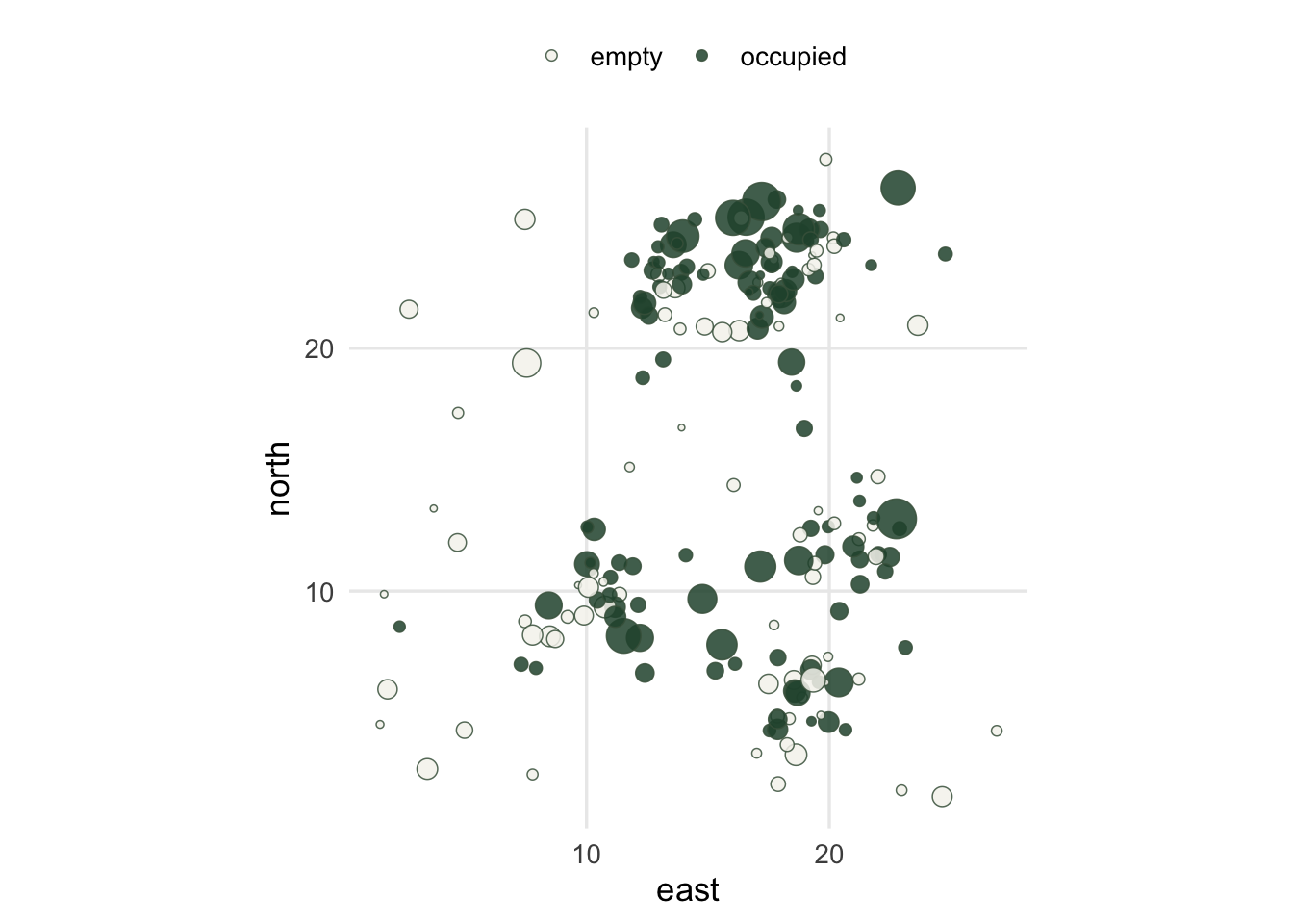
Of the `r n` patches, `r n_occ` are occupied in this snapshot. Occupied patches are larger than empty ones (median area `r round(median(A[o==1]),2)` against `r round(median(A[o==0]),2)`), the fingerprint of the extinction-area relationship.
```{r}
#| label: fig-map
#| fig-cap: "The patch network at a single point in time. Points are patches, sized by area; filled points are occupied and open points empty. Occupation concentrates in the large, well-connected patches of the clusters and thins out among the small isolated patches."
#| fig-alt: "A scatter of circles across a square landscape, in several dense groups and some scattered singletons. Larger circles are more often filled dark green; small circles are mostly open."
#| echo: false
#| warning: false
library(ggplot2)
te_canvas <- theme(plot.background = element_rect(fill = "#f5f4ee", colour = NA),
panel.background = element_rect(fill = "#f5f4ee", colour = NA))
dfm <- data.frame(x = patch[, 1], y = patch[, 2], area = A,
state = ifelse(o == 1L, "occupied", "empty"))
ggplot(dfm, aes(x, y, size = area, fill = state)) +
geom_point(shape = 21, colour = "#46604a", stroke = 0.4, alpha = 0.85) +
scale_size_area(max_size = 7, guide = "none") +
scale_fill_manual(values = c(occupied = "#275139", empty = "#f5f4ee"), name = NULL) +
coord_equal() +
labs(x = "east", y = "north") +
theme_minimal(base_size = 13) + te_canvas +
theme(panel.grid.minor = element_blank(), legend.position = "top")
```
## Fitting the model from the snapshot
We fix `alpha` at 0.6 and estimate the remaining three parameters. Fixing the dispersal parameter is standard practice: it is only weakly identified from a single snapshot, and field studies usually pin it down from independent mark-recapture of dispersers. The checking tutorial returns to why a snapshot cannot say much about `alpha`. The rest is a Bernoulli log-likelihood, maximised with `optim`.
```{r}
#| label: fit
af <- 0.6
S_obs <- conn(o, D, A, af)
nll <- function(p) {
  mu <- exp(p[1]); x <- exp(p[2]); y <- exp(p[3])
  C <- Cfun(S_obs, y); E <- Efun(A, mu, x)
  J <- pmin(pmax(C / (C + E), 1e-9), 1 - 1e-9)
  -sum(dbinom(o, 1, J, log = TRUE))
}
fit <- optim(log(c(0.5, 1, 2)), nll, method = "Nelder-Mead",
             control = list(maxit = 4000, reltol = 1e-12))
fit <- optim(fit$par, nll, method = "BFGS")
ph <- exp(fit$par)
mle <- -fit$value
setNames(round(ph, 3), c("mu", "x", "y"))
```
The point estimates are `mu` = `r round(ph[1],3)`, `x` = `r round(ph[2],3)`, `y` = `r round(ph[3],3)`. One snapshot is a single noisy realisation, so read them alongside their uncertainty. Profile-likelihood intervals make that uncertainty honest.
```{r}
#| label: profile
prof <- function(idx) {
  g <- seq(log(0.05), log(30), length = 200)
  starts <- c(list(fit$par[-idx]),   # the fit, then a spread of starts for the other two
              asplit(as.matrix(expand.grid(log(c(0.2, 1, 5)), log(c(0.2, 1, 5)))), 1))
  pll <- function(v) {
    f <- function(q) { pp <- numeric(3); pp[idx] <- v; pp[-idx] <- q; nll(pp) }
    -min(sapply(starts, function(s) optim(optim(s, f)$par, f, method = "BFGS")$value))
  }
  ll <- sapply(g, pll)
  ok <- which(ll >= mle - 1.92)
  cross <- function(v) pll(v) - (mle - 1.92)   # each end lies between two grid points
  c(exp(uniroot(cross, g[c(min(ok) - 1, min(ok))], tol = 1e-8)$root),
    exp(uniroot(cross, g[c(max(ok), max(ok) + 1)], tol = 1e-8)$root))
}
ci <- t(sapply(1:3, prof))
rownames(ci) <- c("mu", "x", "y"); colnames(ci) <- c("lower", "upper")
round(ci, 3)
```
The profile intervals are `mu` in [`r round(ci[1,1],3)`, `r round(ci[1,2],3)`], `x` in [`r round(ci[2,1],3)`, `r round(ci[2,2],3)`], `y` in [`r round(ci[3,1],3)`, `r round(ci[3,2],3)`].
Does connectivity earn its place? Drop it (force colonisation to one, so incidence depends on area alone) and compare fits. The area-only likelihood has more than one local maximum, so it is fitted from several starts and the best one is kept.
```{r}
#| label: lrt
nll_area <- function(p) {
  mu <- exp(p[1]); x <- exp(p[2])
  E <- Efun(A, mu, x)
  J <- pmin(pmax(1 / (1 + E), 1e-9), 1 - 1e-9)
  -sum(dbinom(o, 1, J, log = TRUE))
}
starts0 <- list(log(c(0.5, 1)), log(c(2, 2)), log(c(10, 4)))
fits0 <- lapply(starts0, function(s) optim(s, nll_area, method = "BFGS"))
fit0 <- fits0[[which.min(sapply(fits0, `[[`, "value"))]]
dev <- 2 * (fit0$value - (-mle))
p_lrt <- pchisq(dev, df = 1, lower.tail = FALSE)
c(deviance = dev, p_value = p_lrt)
```
Adding connectivity improves the fit by a deviance of `r round(dev,1)` on one degree of freedom (p = `r sci_tex(p_lrt, 1)`). That is a boundary test: forcing colonisation to one puts the parameter at the edge of its space, where the reference distribution is a half-and-half mixture of a point mass and chi-squared on one degree of freedom, so the nominal p-value is conservative by about a factor of two. At this deviance it makes no difference to the reading. The colonisation-connectivity relationship is real: isolated patches with very low connectivity have sharply lower incidence, and that is what the likelihood detects.
## The fitted incidence
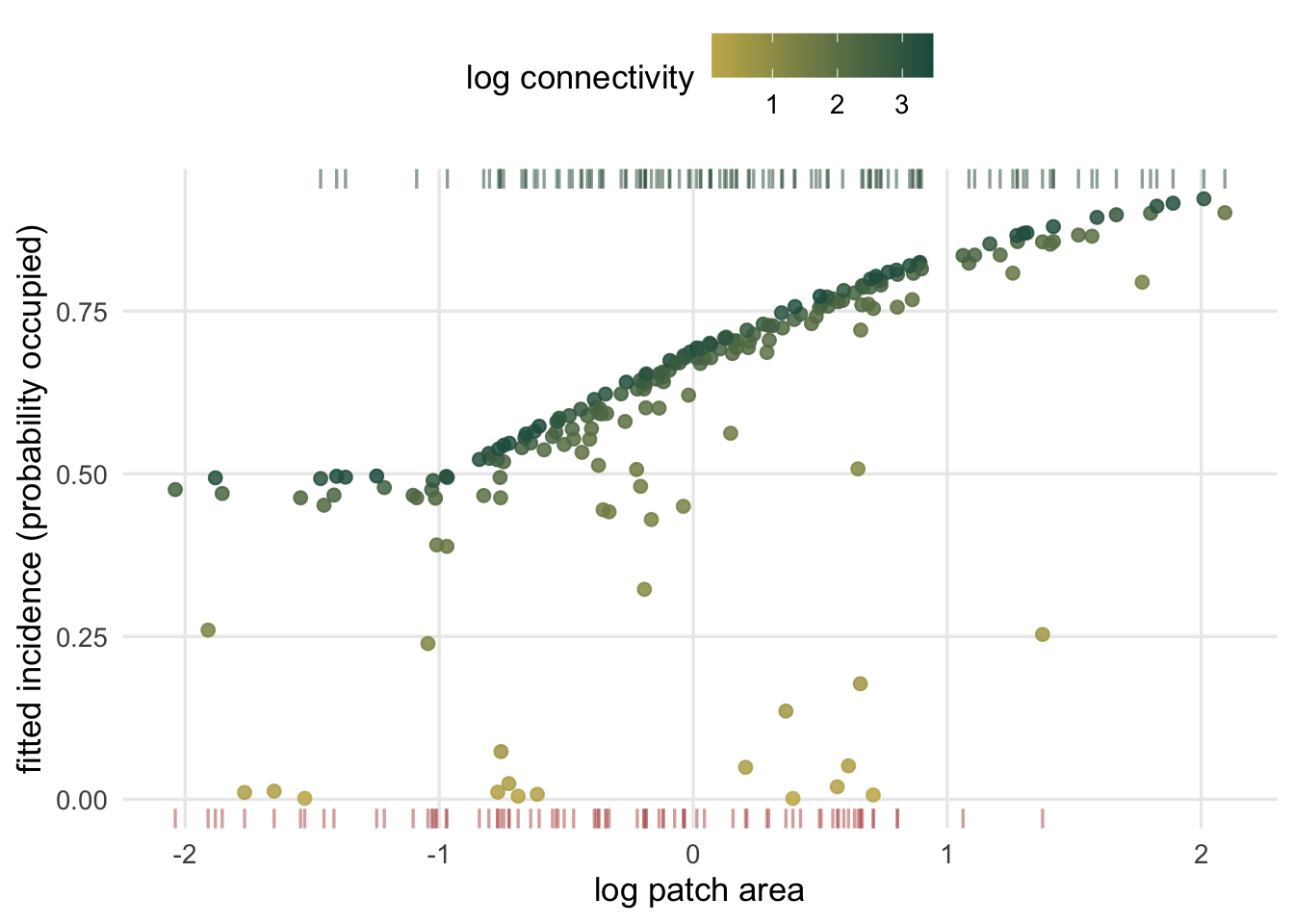
The payoff is a probability of occupancy for every patch, from its area and its connectivity. Plotting the fitted incidence against area shows extinction at work (incidence climbs with area), while the vertical spread at any given area is the connectivity effect.
```{r}
#| label: incidence
mu <- ph[1]; x <- ph[2]; y <- ph[3]
S <- conn(o, D, A, af)
C <- Cfun(S, y); E <- Efun(A, mu, x)
J <- C / (C + E)
acc <- mean((J > 0.5) == o)
c(mean_J_occupied = mean(J[o == 1]), mean_J_empty = mean(J[o == 0]), accuracy = acc)
```
Occupied patches carry a mean fitted incidence of `r round(mean(J[o==1]),3)` against `r round(mean(J[o==0]),3)` for empty ones, and classifying a patch as occupied when its incidence exceeds one half is right `r round(100*acc,0)`% of the time. A snapshot never predicts occupancy exactly, because occupancy is itself stochastic.
```{r}
#| label: fig-incidence
#| fig-cap: "Fitted incidence against patch area, coloured by connectivity. Incidence rises with area (the extinction effect); at any area, better-connected patches sit higher (the colonisation effect). Points along the top and bottom mark patches observed occupied and empty."
#| fig-alt: "Points sit on a flat band just below one half at small log-area, then rise along a curve to high incidence at large log-area, with a scatter of poorly connected points near zero at small and middling areas; darker points (high connectivity) sit above paler ones. A rug of occupied points lines the top and empty points the bottom."
#| echo: false
#| warning: false
dfi <- data.frame(area = A, J = J, conn = S, occ = o)
ggplot(dfi, aes(log(area), J)) +
geom_point(aes(colour = log1p(conn)), size = 2, alpha = 0.85) +
scale_colour_gradient(low = "#c9b458", high = "#1d5b4e", name = "log connectivity") +
geom_rug(data = subset(dfi, occ == 1), sides = "t", colour = "#275139", alpha = 0.5) +
geom_rug(data = subset(dfi, occ == 0), sides = "b", colour = "#b5534e", alpha = 0.5) +
labs(x = "log patch area", y = "fitted incidence (probability occupied)") +
theme_minimal(base_size = 13) + te_canvas +
theme(panel.grid.minor = element_blank(), legend.position = "top")
```
## The bridge, and what the fit assumes
The incidence function model is close kin to the dynamic occupancy models used with repeat surveys. Both estimate a colonisation probability and an extinction probability. The difference is the information they lean on. A dynamic occupancy model watches sites across several seasons and uses that time series (plus a detection layer) to separate the two rates; the incidence function model has only one snapshot in space, so it uses the spatial structure instead, letting area carry the extinction signal and connectivity carry the colonisation signal. Time in one, space in the other, for the same two quantities.
That substitution has a price, and the checking tutorial spends its effort there. Two assumptions do the heavy lifting. The snapshot must be at equilibrium: if the network is recovering from a crash or declining after habitat loss, the pattern reflects transient history rather than the balance of `C` and `E`, and the fit is biased. And the dispersal parameter, fixed here, is barely visible in a snapshot, yet the conservation conclusions of the next tutorial hinge on it. A model this convenient deserves those checks.
## References
Hanski I 1994. Journal of Animal Ecology 63(1):151-162 (10.2307/5591).
Hanski I 1994. Trends in Ecology and Evolution 9(4):131-135 (10.1016/0169-5347(94)90177-5).
Moilanen A 1999. Ecology 80(3):1031-1043 (10.1890/0012-9658(1999)080[1031:POMOMD]2.0.CO;2).
Hanski I 1999. Metapopulation Ecology. Oxford University Press. ISBN 978-0-19-854065-6.
MacKenzie DI, Nichols JD, Hines JE, Knutson MG, Franklin AB 2003. Ecology 84(8):2200-2207 (10.1890/02-3090).
## Related tutorials
- [The Levins metapopulation model](../the-levins-metapopulation-model/)
- [Metapopulation capacity](../metapopulation-capacity/)
- [Checking a metapopulation model](../checking-a-metapopulation-model/)
- [Single-season occupancy models](../single-season-occupancy-model/)