The Levins metapopulation model

metapopulation

population dynamics

ecology tutorial

The Levins model of patch occupancy from scratch in R: the colonisation-extinction balance, the equilibrium fraction, and the extinction threshold.

Author

Tidy Ecology

Published

2026-07-21

A single population lives or dies. A set of populations linked by dispersal can do something a single one cannot: persist as a whole while any one patch winks out, because empty patches get recolonised from occupied ones. Richard Levins wrote down the simplest model of this idea in 1969, and it still frames how ecologists think about fragmented habitats. This post builds the Levins model in base R, finds its equilibrium, fits its two rates from a simulated patch history, and shows the extinction threshold that separates a persisting network from a doomed one.

The model tracks one number: p, the fraction of habitat patches that are occupied. Two processes push it. Occupied patches send out colonists that can settle empty patches, at a rate set by a colonisation parameter c; and occupied patches go locally extinct at a rate e. Patches are treated as identical and equally reachable (the mean-field assumption we return to at the end). The rate of change is

\[\frac{dp}{dt} = c\,p\,(1-p) - e\,p.\]

The colonisation term is c p (1-p): it needs occupied patches to supply colonists (the p) and empty patches to receive them (the 1-p). The extinction term e p just removes a fraction of the occupied patches. That is the whole model.

The equilibrium and the threshold

Set the rate of change to zero. Either p = 0, or the bracket vanishes: c(1-p) - e = 0, which rearranges to

\[p^\* = 1 - \frac{e}{c}.\]

So a metapopulation settles at an occupied fraction that depends only on the ratio of extinction to colonisation. If colonisation comfortably beats extinction, most patches stay filled; as the ratio e/c climbs toward one, the equilibrium slides toward zero. And once e >= c, the formula would give a negative fraction, which is impossible: the only equilibrium left is p* = 0. That is the extinction threshold. A metapopulation persists if and only if e/c < 1.

Notice what the threshold does not say. It does not require every patch to survive; patches keep going extinct at equilibrium. It requires only that colonisation refills them fast enough on average.

c_col <- 0.40    # colonisation parameter
e_ext <- 0.15    # extinction parameter
p_star <- 1 - e_ext / c_col
p_star

[1] 0.625

With these rates the equilibrium is 0.625. Let us confirm it two ways: by iterating the deterministic model, and by simulating patches one at a time.

Iterating the deterministic model

In discrete time the model steps as p_{t+1} = p_t + c p_t (1 - p_t) - e p_t. Starting from a rare metapopulation (one patch in ten occupied), it climbs to the equilibrium and stays there.

levins_map <- function(p0, cc, ee, steps) {
  p <- numeric(steps + 1)
  p[1] <- p0
  for (t in 1:steps) {
    pt <- p[t]
    p[t + 1] <- pt + cc * pt * (1 - pt) - ee * pt
  }
  p
}
steps <- 100
det <- levins_map(p0 = 0.10, cc = c_col, ee = e_ext, steps = steps)
det_final <- det[steps + 1]
det_final

[1] 0.625

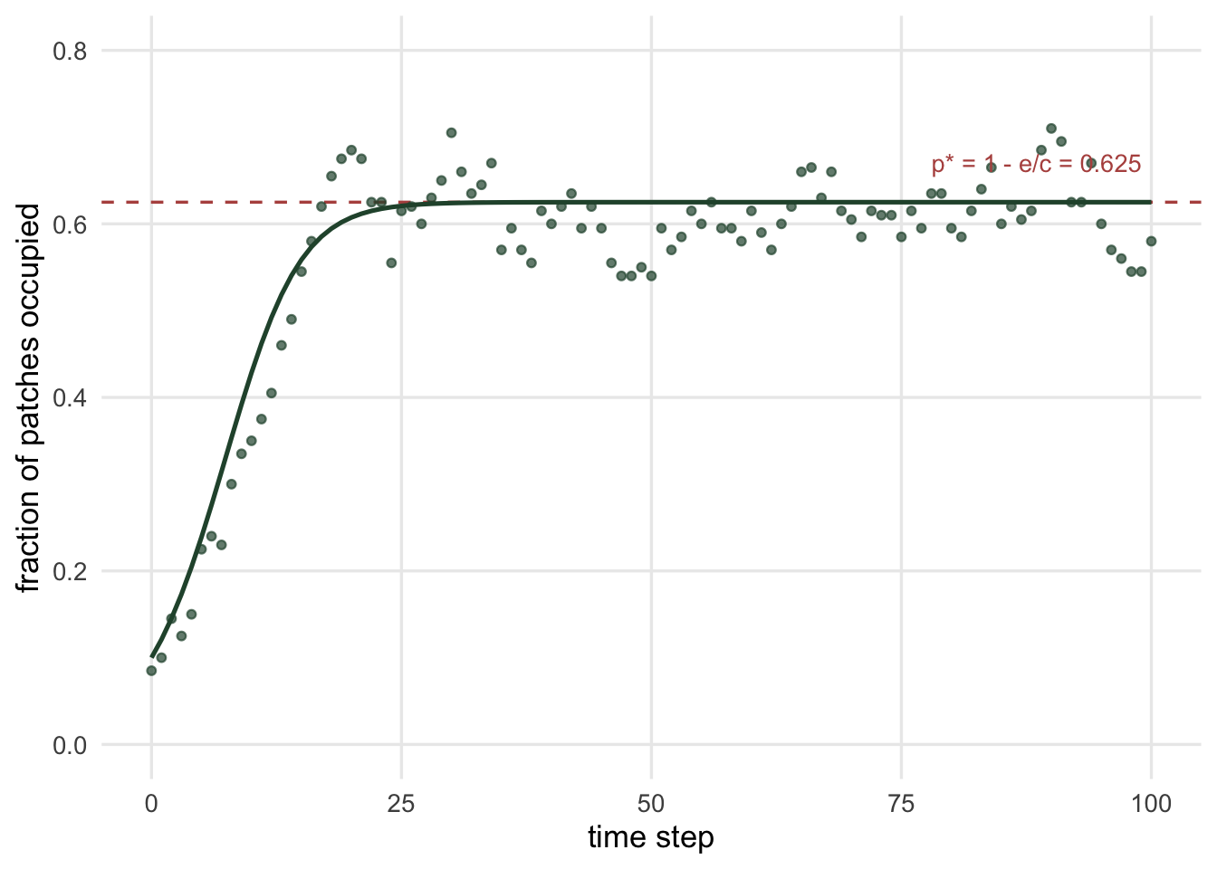
The deterministic trajectory lands on 0.625, exactly p*.

Simulating patches, then recovering the rates

The deterministic curve hides the fact that patches are discrete and stochastic. Let us simulate 200 individual patches. Each time step, an empty patch is colonised with probability c times the current occupied fraction, and an occupied patch survives with probability 1 - e.

sim_patches <- function(n, cc, ee, steps, p0, seed) {
  set.seed(seed)
  occ <- matrix(0L, n, steps + 1)
  occ[, 1] <- as.integer(runif(n) < p0)
  frac <- numeric(steps + 1)
  frac[1] <- mean(occ[, 1])
  for (t in 1:steps) {
    pt <- frac[t]
    st <- occ[, t]
    new <- st
    empty <- st == 0L
    occupied <- st == 1L
    new[empty] <- as.integer(runif(sum(empty)) < cc * pt)
    new[occupied] <- as.integer(runif(sum(occupied)) >= ee)
    occ[, t + 1] <- new
    frac[t + 1] <- mean(new)
  }
  list(occ = occ, frac = frac)
}
n <- 200
sim <- sim_patches(n, c_col, e_ext, steps, p0 = 0.10, seed = 42)
obs_eq <- mean(sim$frac[(steps - 40 + 1):(steps + 1)])
obs_eq

[1] 0.6162195

The stochastic occupied fraction, averaged over the last 40 steps, is 0.616: close to the predicted 0.625, with the wobble you expect from a finite number of patches.

A scatter of points and a smooth solid line both rise steeply from an occupied fraction near 0.1 and level off, oscillating around a horizontal dashed line at 0.625 across 100 time steps. — Figure 1: The occupied fraction of 200 patches climbing from a rare start to the Levins equilibrium. The stochastic realisation (points) tracks the deterministic curve (solid) and settles around the equilibrium p-star = 0.625 (dashed).

The two rates are not just inputs; they are estimable. Given the full patch-by-time occupancy matrix, the log-likelihood is a sum of Bernoulli terms: each empty patch either got colonised or not (probability c times the occupied fraction), and each occupied patch either survived or went extinct (probability e). Maximising it recovers c and e.

occ <- sim$occ
fr <- sim$frac
nll <- function(par) {
  cc <- par[1]; ee <- par[2]
  ll <- 0
  for (t in 1:steps) {
    pt <- fr[t]
    st <- occ[, t]; nx <- occ[, t + 1]
    empty <- st == 0L; occupied <- st == 1L
    cp <- cc * pt
    ll <- ll + sum(dbinom(nx[empty], 1, cp, log = TRUE))
    ll <- ll + sum(dbinom(1L - nx[occupied], 1, ee, log = TRUE))
  }
  -ll
}
fit <- optim(c(0.3, 0.2), nll, method = "L-BFGS-B",
             lower = c(1e-3, 1e-3), upper = c(0.999, 0.999))
c_hat <- fit$par[1]
e_hat <- fit$par[2]
c(c_hat = c_hat, e_hat = e_hat, p_star_hat = 1 - e_hat / c_hat)

     c_hat      e_hat p_star_hat 
 0.4138834  0.1593947  0.6148802

The fit returns c = 0.414 and e = 0.159, close to the true 0.40 and 0.15, and an implied equilibrium of 0.615. The extinction rate has a tidy closed form: it is just the number of extinction events divided by the number of occupied-patch time steps, which comes to 0.159, matching the optimiser exactly.

The threshold in a picture

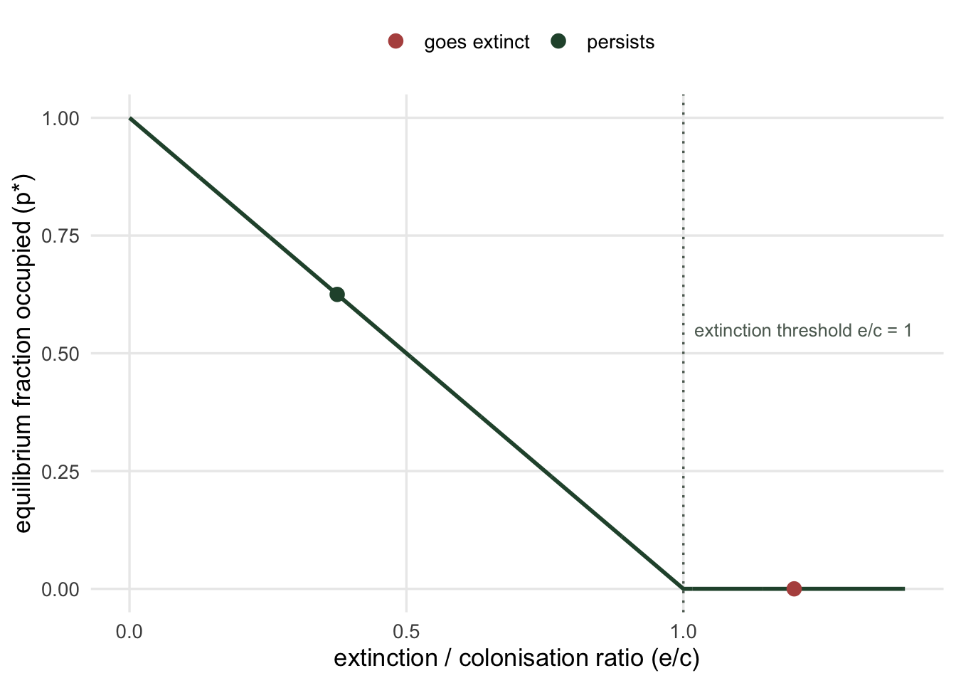
The equilibrium p* = 1 - e/c is a straight fall against the ratio e/c, hitting zero at the threshold. Below it, a fixed fraction of patches stays occupied; at or above it, the whole network drifts to extinction even though individual patches remain perfectly colonisable.

sim_frac <- function(n, cc, ee, steps, p0, seed) {
  set.seed(seed)
  st <- as.integer(runif(n) < p0)
  frac <- numeric(steps + 1); frac[1] <- mean(st)
  for (t in 1:steps) {
    pt <- frac[t]
    empty <- st == 0L; occupied <- st == 1L
    new <- st
    new[empty] <- as.integer(runif(sum(empty)) < cc * pt)
    new[occupied] <- as.integer(runif(sum(occupied)) >= ee)
    st <- new; frac[t + 1] <- mean(st)
  }
  frac
}
c2 <- 0.25; e2 <- 0.30           # e/c = 1.2, above threshold
ratio2 <- e2 / c2
fr_ext <- sim_frac(200, c2, e2, 60, p0 = 0.50, seed = 7)
occ40 <- fr_ext[41]
ratio2

[1] 1.2

occ40

[1] 0.015

With e/c = 1.2 the network starts from half its patches occupied and collapses: by step 40 only 0.015 of patches remain occupied, and it reaches zero soon after. Colonisation never stopped; it simply could not keep pace with extinction.

A line falls linearly from an occupied fraction of 1 at ratio zero to zero at ratio one, then stays flat at zero. A green point sits at ratio 0.375 and a red point at ratio 1.2 on the flat part. — Figure 2: Equilibrium occupancy as a function of the extinction-to-colonisation ratio. The metapopulation persists only where e/c is below one; at and beyond the threshold the equilibrium is zero. Points mark the two scenarios simulated above.

What the mean-field model leaves out

The Levins model is a starting point, not a finished tool, and its simplicity comes from two assumptions worth naming. Every patch is treated as identical, so a tiny patch and a large one have the same extinction rate; and colonisation is spatially implicit, so every occupied patch is an equally good source for every empty one no matter how far apart they sit. Real fragmented landscapes break both: extinction risk falls with patch area, and a colonist is far more likely to reach a nearby patch than a distant one. The next tutorial, on the incidence function model, keeps the colonisation-extinction logic but lets patch area drive extinction and lets distance drive colonisation, so the model can be fitted to a real map of patches. A third assumption is quieter: the estimate of c and e above used the full time series of who was occupied when. With only a single snapshot in time, recovering the two rates is harder, and it leans on the network sitting at its equilibrium; that is where the incidence function model and its checks earn their keep.

One more caution sits in the threshold itself. e/c < 1 is a statement about long-run averages in an infinitely large network. A finite, stochastic metapopulation can drift to extinction by chance even when the deterministic model says it should persist, a point the checking tutorial makes concrete.

References

Levins R 1969. Bulletin of the Entomological Society of America 15(3):237-240 (10.1093/besa/15.3.237).

Gotelli NJ 1991. The American Naturalist 138(3):768-776 (10.1086/285249).

Hanski I 1998. Nature 396:41-49 (10.1038/23876).

--- title: "The Levins metapopulation model" description: "The Levins model of patch occupancy from scratch in R: the colonisation-extinction balance, the equilibrium fraction, and the extinction threshold." date: "2026-07-21 09:00" categories: [R, metapopulation, population dynamics, ecology tutorial] image: thumbnail.png image-alt: "A line rising from low occupancy toward a dashed equilibrium at 0.625, next to a curve of equilibrium occupancy falling to zero at an extinction threshold." --- A single population lives or dies. A set of populations linked by dispersal can do something a single one cannot: persist as a whole while any one patch winks out, because empty patches get recolonised from occupied ones. Richard Levins wrote down the simplest model of this idea in 1969, and it still frames how ecologists think about fragmented habitats. This post builds the Levins model in base R, finds its equilibrium, fits its two rates from a simulated patch history, and shows the extinction threshold that separates a persisting network from a doomed one. The model tracks one number: `p`, the fraction of habitat patches that are occupied. Two processes push it. Occupied patches send out colonists that can settle empty patches, at a rate set by a colonisation parameter `c`; and occupied patches go locally extinct at a rate `e`. Patches are treated as identical and equally reachable (the mean-field assumption we return to at the end). The rate of change is $$\frac{dp}{dt} = c\,p\,(1-p) - e\,p.$$ The colonisation term is `c p (1-p)`: it needs occupied patches to supply colonists (the `p`) and empty patches to receive them (the `1-p`). The extinction term `e p` just removes a fraction of the occupied patches. That is the whole model. ## The equilibrium and the threshold Set the rate of change to zero. Either `p = 0`, or the bracket vanishes: `c(1-p) - e = 0`, which rearranges to $$p^\* = 1 - \frac{e}{c}.$$ So a metapopulation settles at an occupied fraction that depends only on the ratio of extinction to colonisation. If colonisation comfortably beats extinction, most patches stay filled; as the ratio `e/c` climbs toward one, the equilibrium slides toward zero. And once `e >= c`, the formula would give a negative fraction, which is impossible: the only equilibrium left is `p* = 0`. That is the extinction threshold. A metapopulation persists if and only if `e/c < 1`. Notice what the threshold does not say. It does not require every patch to survive; patches keep going extinct at equilibrium. It requires only that colonisation refills them fast enough on average. ```{r} #| label: params c_col <- 0.40 # colonisation parameter e_ext <- 0.15 # extinction parameter p_star <- 1 - e_ext / c_col p_star ``` With these rates the equilibrium is `r round(p_star, 3)`. Let us confirm it two ways: by iterating the deterministic model, and by simulating patches one at a time. ## Iterating the deterministic model In discrete time the model steps as `p_{t+1} = p_t + c p_t (1 - p_t) - e p_t`. Starting from a rare metapopulation (one patch in ten occupied), it climbs to the equilibrium and stays there. ```{r} #| label: deterministic levins_map <- function(p0, cc, ee, steps) { p <- numeric(steps + 1) p[1] <- p0 for (t in 1:steps) { pt <- p[t] p[t + 1] <- pt + cc * pt * (1 - pt) - ee * pt } p } steps <- 100 det <- levins_map(p0 = 0.10, cc = c_col, ee = e_ext, steps = steps) det_final <- det[steps + 1] det_final ``` The deterministic trajectory lands on `r round(det_final, 3)`, exactly `p*`. ## Simulating patches, then recovering the rates The deterministic curve hides the fact that patches are discrete and stochastic. Let us simulate 200 individual patches. Each time step, an empty patch is colonised with probability `c` times the current occupied fraction, and an occupied patch survives with probability `1 - e`. ```{r} #| label: simulate sim_patches <- function(n, cc, ee, steps, p0, seed) { set.seed(seed) occ <- matrix(0L, n, steps + 1) occ[, 1] <- as.integer(runif(n) < p0) frac <- numeric(steps + 1) frac[1] <- mean(occ[, 1]) for (t in 1:steps) { pt <- frac[t] st <- occ[, t] new <- st empty <- st == 0L occupied <- st == 1L new[empty] <- as.integer(runif(sum(empty)) < cc * pt) new[occupied] <- as.integer(runif(sum(occupied)) >= ee) occ[, t + 1] <- new frac[t + 1] <- mean(new) } list(occ = occ, frac = frac) } n <- 200 sim <- sim_patches(n, c_col, e_ext, steps, p0 = 0.10, seed = 42) obs_eq <- mean(sim$frac[(steps - 40 + 1):(steps + 1)]) obs_eq ``` The stochastic occupied fraction, averaged over the last 40 steps, is `r round(obs_eq, 3)`: close to the predicted `r round(p_star, 3)`, with the wobble you expect from a finite number of patches. ```{r} #| label: fig-trajectory #| fig-cap: "The occupied fraction of 200 patches climbing from a rare start to the Levins equilibrium. The stochastic realisation (points) tracks the deterministic curve (solid) and settles around the equilibrium p-star = 0.625 (dashed)." #| fig-alt: "A scatter of points and a smooth solid line both rise steeply from an occupied fraction near 0.1 and level off, oscillating around a horizontal dashed line at 0.625 across 100 time steps." #| echo: false #| warning: false library(ggplot2) dfp <- data.frame(t = 0:steps, stoch = sim$frac, det = det) ggplot(dfp, aes(t)) + geom_hline(yintercept = p_star, linetype = "dashed", colour = "#b5534e", linewidth = 0.6) + geom_point(aes(y = stoch), colour = "#275139", size = 1.3, alpha = 0.7) + geom_line(aes(y = det), colour = "#275139", linewidth = 0.9) + annotate("text", x = 78, y = p_star + 0.045, label = "p* = 1 - e/c = 0.625", colour = "#b5534e", size = 3.6, hjust = 0) + labs(x = "time step", y = "fraction of patches occupied") + coord_cartesian(ylim = c(0, 0.8)) + theme_minimal(base_size = 13) + theme(panel.grid.minor = element_blank()) ``` The two rates are not just inputs; they are estimable. Given the full patch-by-time occupancy matrix, the log-likelihood is a sum of Bernoulli terms: each empty patch either got colonised or not (probability `c` times the occupied fraction), and each occupied patch either survived or went extinct (probability `e`). Maximising it recovers `c` and `e`. ```{r} #| label: fit occ <- sim$occ fr <- sim$frac nll <- function(par) { cc <- par[1]; ee <- par[2] ll <- 0 for (t in 1:steps) { pt <- fr[t] st <- occ[, t]; nx <- occ[, t + 1] empty <- st == 0L; occupied <- st == 1L cp <- cc * pt ll <- ll + sum(dbinom(nx[empty], 1, cp, log = TRUE)) ll <- ll + sum(dbinom(1L - nx[occupied], 1, ee, log = TRUE)) } -ll } fit <- optim(c(0.3, 0.2), nll, method = "L-BFGS-B", lower = c(1e-3, 1e-3), upper = c(0.999, 0.999)) c_hat <- fit$par[1] e_hat <- fit$par[2] c(c_hat = c_hat, e_hat = e_hat, p_star_hat = 1 - e_hat / c_hat) ``` The fit returns `c` = `r round(c_hat, 3)` and `e` = `r round(e_hat, 3)`, close to the true 0.40 and 0.15, and an implied equilibrium of `r round(1 - e_hat / c_hat, 3)`. The extinction rate has a tidy closed form: it is just the number of extinction events divided by the number of occupied-patch time steps, which comes to `r round(sum(occ[, 1:steps] == 1L & occ[, 2:(steps + 1)] == 0L) / sum(occ[, 1:steps]), 3)`, matching the optimiser exactly. ## The threshold in a picture The equilibrium `p* = 1 - e/c` is a straight fall against the ratio `e/c`, hitting zero at the threshold. Below it, a fixed fraction of patches stays occupied; at or above it, the whole network drifts to extinction even though individual patches remain perfectly colonisable. ```{r} #| label: extinction-sim sim_frac <- function(n, cc, ee, steps, p0, seed) { set.seed(seed) st <- as.integer(runif(n) < p0) frac <- numeric(steps + 1); frac[1] <- mean(st) for (t in 1:steps) { pt <- frac[t] empty <- st == 0L; occupied <- st == 1L new <- st new[empty] <- as.integer(runif(sum(empty)) < cc * pt) new[occupied] <- as.integer(runif(sum(occupied)) >= ee) st <- new; frac[t + 1] <- mean(st) } frac } c2 <- 0.25; e2 <- 0.30 # e/c = 1.2, above threshold ratio2 <- e2 / c2 fr_ext <- sim_frac(200, c2, e2, 60, p0 = 0.50, seed = 7) occ40 <- fr_ext[41] ratio2 occ40 ``` With `e/c` = `r round(ratio2, 2)` the network starts from half its patches occupied and collapses: by step 40 only `r round(occ40, 3)` of patches remain occupied, and it reaches zero soon after. Colonisation never stopped; it simply could not keep pace with extinction. ```{r} #| label: fig-threshold #| fig-cap: "Equilibrium occupancy as a function of the extinction-to-colonisation ratio. The metapopulation persists only where e/c is below one; at and beyond the threshold the equilibrium is zero. Points mark the two scenarios simulated above." #| fig-alt: "A line falls linearly from an occupied fraction of 1 at ratio zero to zero at ratio one, then stays flat at zero. A green point sits at ratio 0.375 and a red point at ratio 1.2 on the flat part." #| echo: false #| warning: false rr <- seq(0, 1.4, by = 0.001) dft <- data.frame(ratio = rr, pstar = pmax(0, 1 - rr)) pts <- data.frame(ratio = c(e_ext / c_col, ratio2), pstar = c(p_star, 0), lab = c("persists", "goes extinct")) ggplot(dft, aes(ratio, pstar)) + geom_vline(xintercept = 1, linetype = "dotted", colour = "#5d6b61") + geom_line(colour = "#275139", linewidth = 1) + geom_point(data = pts, aes(colour = lab), size = 3) + scale_colour_manual(values = c(persists = "#275139", `goes extinct` = "#b5534e"), name = NULL) + annotate("text", x = 1.02, y = 0.55, label = "extinction threshold e/c = 1", colour = "#5d6b61", size = 3.4, hjust = 0) + labs(x = "extinction / colonisation ratio (e/c)", y = "equilibrium fraction occupied (p*)") + theme_minimal(base_size = 13) + theme(panel.grid.minor = element_blank(), legend.position = "top") ``` ## What the mean-field model leaves out The Levins model is a starting point, not a finished tool, and its simplicity comes from two assumptions worth naming. Every patch is treated as identical, so a tiny patch and a large one have the same extinction rate; and colonisation is spatially implicit, so every occupied patch is an equally good source for every empty one no matter how far apart they sit. Real fragmented landscapes break both: extinction risk falls with patch area, and a colonist is far more likely to reach a nearby patch than a distant one. The next tutorial, on the incidence function model, keeps the colonisation-extinction logic but lets patch area drive extinction and lets distance drive colonisation, so the model can be fitted to a real map of patches. A third assumption is quieter: the estimate of `c` and `e` above used the full time series of who was occupied when. With only a single snapshot in time, recovering the two rates is harder, and it leans on the network sitting at its equilibrium; that is where the incidence function model and its checks earn their keep. One more caution sits in the threshold itself. `e/c < 1` is a statement about long-run averages in an infinitely large network. A finite, stochastic metapopulation can drift to extinction by chance even when the deterministic model says it should persist, a point the checking tutorial makes concrete. ## References Levins R 1969. Bulletin of the Entomological Society of America 15(3):237-240 (10.1093/besa/15.3.237). Gotelli NJ 1991. The American Naturalist 138(3):768-776 (10.1086/285249). Hanski I 1998. Nature 396:41-49 (10.1038/23876). ## Related tutorials - [The incidence function model](../incidence-function-model/) - [Metapopulation capacity](../metapopulation-capacity/) - [Checking a metapopulation model](../checking-a-metapopulation-model/) - [Dynamic occupancy: colonisation and extinction](../dynamic-occupancy-colonisation-extinction/)