library(ggplot2)
library(patchwork)

te_paper  <- "#f5f4ee"
te_ink    <- "#16241d"
te_body   <- "#2c3a31"
te_forest <- "#275139"
te_rust   <- "#b5534e"
te_gold   <- "#c9b458"
te_line   <- "#dad9ca"

theme_datasheet <- function() {
  theme_minimal(base_size = 12) +
    theme(plot.background  = element_rect(fill = te_paper, colour = NA),
          panel.background = element_rect(fill = te_paper, colour = NA),
          panel.grid.major = element_line(colour = te_line, linewidth = 0.3),
          panel.grid.minor = element_blank(),
          text             = element_text(colour = te_body),
          plot.title       = element_text(colour = te_ink, face = "bold"),
          plot.subtitle    = element_text(colour = te_body),
          axis.text        = element_text(colour = te_body))
}Island biogeography and turnover
R
biogeography
species richness
community ecology
ecology tutorial
Simulate the MacArthur and Wilson equilibrium in R: island richness settles while the species list keeps changing, and turnover depends on the survey gap.
An island in a bay is surveyed for breeding land birds in one summer and again forty years later. Both surveys come back with about thirty species, and the obvious reading is that nothing happened. Then somebody puts the two lists side by side and finds that half the names are different: species on the first list that no longer breed there, and species on the second list that were not there before.
That is the result MacArthur and Wilson (1967) predicted. Immigration of species new to the island falls as the island fills up, because the mainland pool of species not yet present shrinks. Extinction rises as the island fills up, because there are more resident populations available to fail. Richness settles where the two rates cross. At the crossing point the rates are equal and neither is zero, so species keep arriving and keep dying out while the count stays put. The equilibrium is in the number, not in the membership.
This post builds the species level version of that model in base R. Every species in the mainland pool runs its own two state chain, colonising when absent and going extinct when present, so both the richness and the identity of the island’s list fall out as outputs rather than being imposed. Two neighbouring tutorials on this site cover the projections of the same idea and stop short of this one. The species-area relationships post fits the richness curve statically, a power law against Gleason’s logarithmic model, with no process underneath it; the Levins metapopulation model post makes one species’ patch occupancy dynamic, with no richness in it at all. The claim here is that those two are projections of a single dynamic, and that the species replacement running underneath a flat richness is the thing neither of them can see.
An island is one two-state chain per species
The island’s state is one bit per species in the mainland pool: present or absent. An absent species arrives at its own colonisation rate, a present species dies out at its own extinction rate, and species do not interact. Distance enters through colonisation: the rate falls exponentially with the crossing a propagule has to make. Area enters through extinction: a larger island holds larger populations, so the rate falls as a power of area.
Species in a real pool are not interchangeable: some disperse well, some hold on badly. Two lognormal multipliers carry that, one on colonisation and one on extinction, so the pool has good colonists that rarely stay and poor colonists that persist once they arrive.
n_pool  <- 80
c_base  <- 0.12     # colonisation rate per species per year at zero distance
e_base  <- 0.10     # extinction rate per species per year on a one km2 island
d_scale <- 15       # dispersal kernel scale, km
b_area  <- 0.45     # exponent linking island area to extinction rate

set.seed(4021)
disp  <- exp(rnorm(n_pool, 0, 0.5))
prone <- exp(rnorm(n_pool, 0, 0.5))
col_of <- function(dist_km) c_base * disp * exp(-dist_km / d_scale)
ext_of <- function(area)    e_base * prone * area^(-b_area)
near_km <- 10; far_km <- 20      # crossing distance, km
small_a <- 1;  large_a <- 2      # island area, km2
closed_form <- function(col_rate, ext_rate) {
  p_pres <- col_rate / (col_rate + ext_rate)
  list(rich   = sum(p_pres),
       sd     = sqrt(sum(p_pres * (1 - p_pres))),
       churn  = sum(p_pres * ext_rate),
       relax  = 1 / min(col_rate + ext_rate),
       p_pres = p_pres)
}
ns_col <- col_of(near_km); ns_ext <- ext_of(small_a)
ns_cf  <- closed_form(ns_col, ns_ext)
relax_all <- max(vapply(list(c(near_km, small_a), c(far_km, small_a),
                            c(near_km, large_a), c(far_km, large_a)),
                        function(v) closed_form(col_of(v[1]), ext_of(v[2]))$relax, 0))
Because the species are independent, the whole equilibrium is available in closed form and nothing has to be simulated to get it. One species is present with probability equal to its colonisation rate divided by the sum of its two rates. Expected richness is the sum of those probabilities, the variance of richness is the sum of each probability times one minus itself, and the rate at which species drop off the list is the sum of each probability times its extinction rate.
For the near, small island that gives an expected richness of 31.8 species out of a pool of 80, a standard deviation of 4.15 species, and an instantaneous loss rate of 3.20 species per year. Those three numbers are the whole of the model, and they are also the target the simulator has to hit before anything else it produces can be believed.
The simulator has to reproduce the algebra before it is used
A two state chain has an exact solution over any interval, so there is no need to chop time into steps small enough to approximate one. If the two rates sum to a total, then the probability that a present species is still present a step later is its stationary probability plus one minus that stationary probability times the exponential decay over the step, and the probability that an absent species has arrived is its stationary probability times one minus the same decay. Those two expressions are exact at the grid points whatever the step size, which means the state of the island at each survey date is drawn from the right distribution even with a step of a whole year.
sim_island <- function(col_rate, ext_rate, n_step, n_rep, dt = 1, from_empty = TRUE) {
  n_sp   <- length(col_rate)
  tot    <- col_rate + ext_rate
  p_pres <- col_rate / tot
  decay  <- exp(-tot * dt)
  p_stay <- p_pres + (1 - p_pres) * decay   # present now, present a step later
  p_gain <- p_pres * (1 - decay)            # absent now, present a step later
  occ <- matrix(if (from_empty) FALSE else runif(n_sp * n_rep) < p_pres, n_sp, n_rep)
  out <- array(FALSE, dim = c(n_sp, n_rep, n_step + 1L))
  out[, , 1] <- occ
  for (k in seq_len(n_step)) {
    thr <- ifelse(occ, p_stay, p_gain)
    occ <- matrix(runif(n_sp * n_rep), n_sp, n_rep) < thr
    out[, , k + 1L] <- occ
  }
  out
}
n_burn <- 200; n_meas <- 400; n_rep <- 40
n_dt <- 12; n_sar_rep <- 20; n_gap_rep <- 30
burn_mult <- n_burn / relax_all
Every island below starts empty, which is the colonisation experiment rather than a convenient initial condition, and the first 200 years are thrown away. That burn-in was fixed before any output was looked at, from the slowest relaxation time in the four islands used later: the sum of the two rates for the most sluggish species implies a relaxation time of 18 years, and 200 years is 11 times that. The replicate count was fixed the same way, from the closed form spread rather than from any output: richness varies by 4.15 species within a run, so 40 independent islands averaged over a 400 year window put the standard error on a mean richness far below the smallest contrast the post goes on to claim. The later experiments use their own counts, 12 runs per step size, 20 per island area and 30 for the survey gap grid, each fixed the same way.
set.seed(801)
occ_ns  <- sim_island(ns_col, ns_ext, n_burn + n_meas, n_rep)
rich_ns <- apply(occ_ns, c(2, 3), sum)
win     <- (n_burn + 1):(n_burn + n_meas + 1)
rep_mean  <- rowMeans(rich_ns[, win])
rich_bar  <- mean(rep_mean); rich_mcse <- sd(rep_mean) / sqrt(n_rep)
rich_sd   <- mean(apply(rich_ns[, win], 1, sd))
band      <- quantile(as.vector(rich_ns[, win]), c(0.05, 0.95))
band_wid  <- unname(band[2] - band[1]); rich_gap <- abs(rich_bar - ns_cf$rich)
The simulated time average is 31.80 species with a Monte Carlo standard error of 0.10, against a closed form value of 31.76, a gap of 0.04 species. The simulated standard deviation of richness within a run is 4.10 against the closed form 4.15. The chain is doing what the algebra says it should.
n_show <- 10; yr_full <- seq_len(ncol(rich_ns)) - 1
appr <- data.frame(year = rep(yr_full, n_show),
                   rich = as.vector(t(rich_ns[seq_len(n_show), ])),
                   run  = factor(rep(seq_len(n_show), each = length(yr_full))))
ggplot(appr, aes(year, rich, group = run)) +
  geom_line(colour = te_forest, alpha = 0.45, linewidth = 0.4) +
  geom_hline(yintercept = ns_cf$rich, colour = te_rust, linewidth = 0.9) +
  geom_vline(xintercept = n_burn, colour = te_gold, linetype = "dashed", linewidth = 0.7) +
  labs(x = "year since the island was bare", y = "species present",
       title = "Filling up, then staying full",
       subtitle = "red: closed form equilibrium; dashed gold: end of burn-in") +
  theme_datasheet()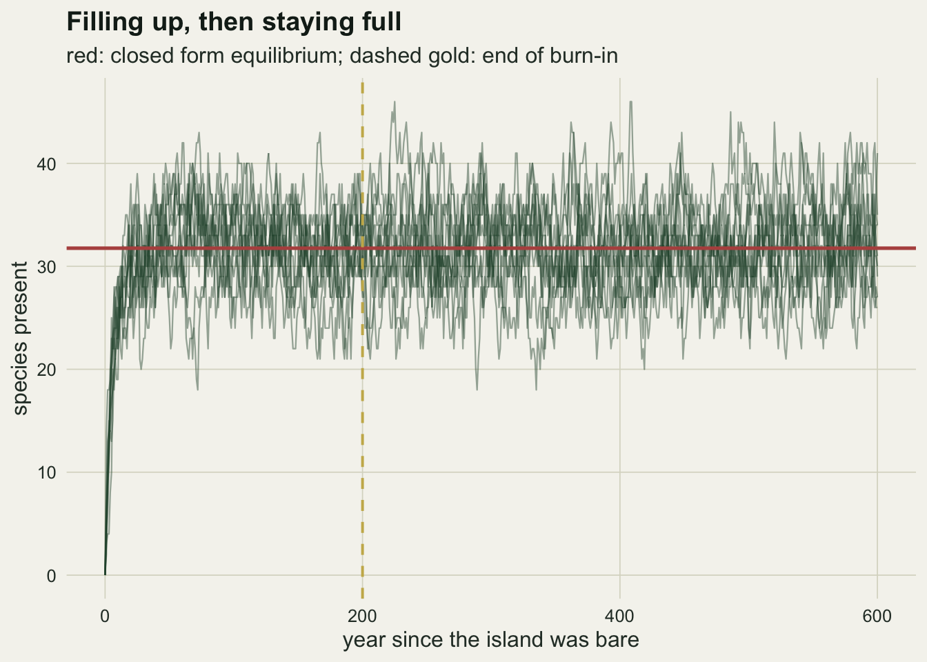
That rise is the shape Simberloff and Wilson (1969) fumigated small mangrove islands to see, and the shape their two year follow up (Simberloff and Wilson 1970) confirmed: arthropod richness climbed back to roughly its pre-treatment level within about a year, while the species making up that richness were not the ones that had been removed.
The second check is about measurement rather than about the chain. The loss rate in the closed form is an instantaneous rate, and a survey run once a year cannot see a species that colonised in March and was gone by November. Counting the disappearances a survey would notice, at four survey intervals, shows how much of the true rate each one recovers.
seen_exact <- function(dt) {
  sum(ns_cf$p_pres * (1 - ns_cf$p_pres) *
      (1 - exp(-(ns_col + ns_ext) * dt))) / dt
}
dt_grid   <- c(1, 0.5, 0.25, 0.125)
exact_rate <- vapply(dt_grid, seen_exact, 0)
set.seed(1207)
seen_rate <- seen_se <- numeric(length(dt_grid))
for (j in seq_along(dt_grid)) {
  d <- dt_grid[j]
  per_run <- vapply(seq_len(n_dt), function(r) {
    oc <- sim_island(ns_col, ns_ext, round((n_burn + 200) / d), 1, dt = d)
    wk <- (round(n_burn / d) + 1):(dim(oc)[3])
    was <- oc[, 1, wk[-length(wk)]]; now <- oc[, 1, wk[-1]]
    sum(was & !now) / (length(wk) - 1) / d
  }, 0)
  seen_rate[j] <- mean(per_run); seen_se[j] <- sd(per_run) / sqrt(n_dt)
}
seen_share <- exact_rate / ns_cf$churn
rel_off    <- abs(seen_rate - exact_rate) / exact_rate
rel_z      <- abs(seen_rate - exact_rate) / seen_se; j_worst <- which.max(rel_off)
sim_gap    <- rel_off[j_worst]; sim_z <- rel_z[j_worst]; dt_worst <- dt_grid[j_worst]
The expected count is available in closed form as well, because the chance that a species present at one survey is absent at the next is its probability of being absent times one minus the decay over the gap. That expectation says an annual survey sees 90.0 per cent of the instantaneous loss rate, and a survey every 0.125 years sees 98.7 per cent. The simulator reproduces that expectation at all four step sizes, with 12 runs behind each: the largest relative discrepancy is 1.0 per cent, at the 0.5 year step, and that same discrepancy is 1.1 Monte Carlo standard errors. Everything below reports the rate a survey at a stated interval would see, never the instantaneous rate, because the instantaneous rate is not observable in the field.
The count is steady and the list is not
Take the near, small island at equilibrium, pick any year as the first survey, and compare it with the survey ten years later. Two quantities come out of that comparison. The gross change is the number of species that switched status in either direction, which is what a field ecologist would call turnover. The net change is the absolute difference in the counts, which is what a richness time series shows.
gap_main <- 10
t_first  <- win[win + gap_main <= max(win)]
gross_v <- net_v <- lost_v <- numeric(0)
for (r in seq_len(n_rep)) {
  was <- occ_ns[, r, t_first]; now <- occ_ns[, r, t_first + gap_main]
  gross_v <- c(gross_v, colSums(was & !now) + colSums(!was & now))
  net_v   <- c(net_v,   abs(colSums(now) - colSums(was)))
  lost_v  <- c(lost_v,  colSums(was & !now) / colSums(was))
}
gross_bar <- mean(gross_v); net_bar <- mean(net_v); lost_bar <- mean(lost_v)
gross_ratio <- gross_bar / net_bar
rep_id     <- rep(seq_len(n_rep), each = length(t_first))
gross_rep  <- tapply(gross_v, rep_id, mean); net_rep <- tapply(net_v, rep_id, mean)
gross_mcse <- sd(gross_rep) / sqrt(n_rep); net_mcse <- sd(net_rep) / sqrt(n_rep)
ratio_mcse <- sd(gross_rep / net_rep) / sqrt(n_rep)
lost_mcse  <- sd(tapply(lost_v, rep_id, mean)) / sqrt(n_rep)
ever_seen <- t(vapply(seq_len(n_rep), function(r) {
  m <- occ_ns[, r, win]
  keep <- rep(FALSE, n_pool)
  vapply(seq_len(ncol(m)), function(k) { keep <<- keep | m[, k]; sum(keep) }, 0)
}, numeric(length(win))))
ever_bar   <- colMeans(ever_seen); yr_century <- 100
ever_100   <- ever_bar[yr_century + 1L]; ever_end <- ever_bar[length(ever_bar)]
Averaged over 40 islands and every starting year in the measurement window, 28.0 species change status across a gap of 10 years, with a Monte Carlo standard error of 0.06, while the count itself moves by 4.3 species plus or minus 0.05, a ratio of 6.6 to one plus or minus 0.08. Of the species present at the first survey, 43.9 per cent are gone by the second, with a Monte Carlo standard error of 0.2 percentage points.
The cumulative list makes the same point from the other side. Standing richness holds at 31.8 species, but the number of distinct species that have been recorded at least once reaches 79 after 100 years of annual surveys and 80 after the full 400 years. An island whose richness sits inside a band of 14 species in nine years out of ten eventually hosts the entire mainland pool.
n_yr_show <- 120; yr_show <- seq_len(n_yr_show + 1) - 1
show_idx  <- win[seq_len(n_yr_show + 1)]
bar <- expand.grid(sp = seq_len(n_pool), year = yr_show)
bar$occ <- as.vector(occ_ns[order(ns_cf$p_pres), 1, show_idx])
p_bar <- ggplot(bar, aes(year, sp, fill = occ)) +
  geom_raster() +
  scale_fill_manual(values = c(`FALSE` = te_line, `TRUE` = te_forest), guide = "none") +
  labs(x = NULL, y = "species, rarest at the bottom",
       title = "Every row is a species, green means present") +
  theme_datasheet() + theme(panel.grid.major = element_blank())

low <- data.frame(year = yr_show, rich = rich_ns[1, show_idx],
                  ever = ever_bar[seq_len(n_yr_show + 1)])
p_low <- ggplot(low, aes(year)) +
  geom_ribbon(aes(ymin = band[1], ymax = band[2]), fill = te_gold, alpha = 0.22) +
  geom_line(aes(y = rich), colour = te_forest, linewidth = 0.8) +
  geom_line(aes(y = ever), colour = te_rust, linewidth = 0.9) +
  labs(x = "year of the equilibrium window", y = "species",
       title = "Flat count, growing list",
       subtitle = paste0("green: one island's richness, gold: its 5 to 95 per cent band\n",
                         "red: distinct species ever recorded, mean of ", n_rep, " islands")) +
  theme_datasheet()

p_bar / p_low + plot_layout(heights = c(1.25, 1)) +
  plot_annotation(theme = theme_datasheet())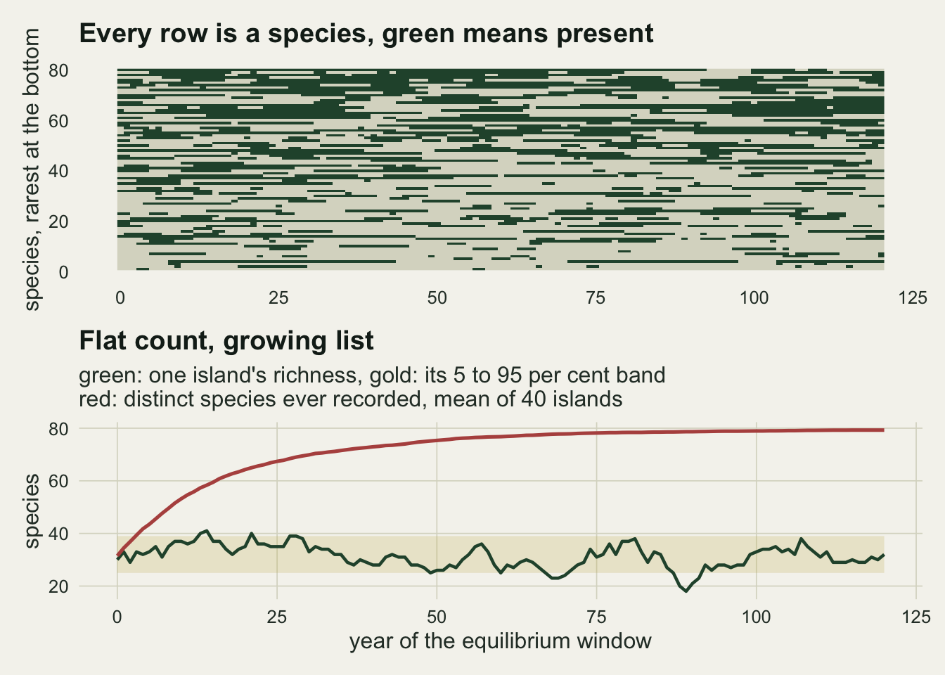
The raster is the argument. Rows near the bottom are poor colonists that are absent most of the time and flicker on briefly; rows near the top are good colonists with low extinction rates that are present in most years but still drop out from time to time. The churn lives in the middle band, and it never stops, while the column sums that make the green line below spend nine years in ten inside the shaded band.
Distance sets the ceiling, area sets the churn
MacArthur and Wilson’s two geographical predictions are separable in this model because distance and area enter different rates. Halving the crossing distance raises every colonisation rate; doubling the area lowers every extinction rate. Four islands, one of each combination, run with the same pool and the same burn-in.
isl_spec <- data.frame(dist_km = c(near_km, far_km, near_km, far_km),
                       area    = c(small_a, small_a, large_a, large_a))
set.seed(902)
isl_out <- do.call(rbind, lapply(seq_len(nrow(isl_spec)), function(i) {
  oc <- sim_island(col_of(isl_spec$dist_km[i]), ext_of(isl_spec$area[i]),
                   n_burn + n_meas, n_rep)
  mu <- rowMeans(apply(oc, c(2, 3), sum)[, win])
  lf <- vapply(seq_len(n_rep), function(r) {
    was <- oc[, r, t_first]; now <- oc[, r, t_first + gap_main]
    sum(was & !now) / sum(was)
  }, 0)
  ann <- vapply(seq_len(n_rep), function(r) {
    was <- oc[, r, win[-length(win)]]; now <- oc[, r, win[-1]]
    mean(colSums(was & !now))
  }, 0)
  data.frame(island = c("near, small", "far, small",
                        "near, large", "far, large")[i],
             rich = mean(mu), rich_se = sd(mu) / sqrt(n_rep),
             lost = 100 * mean(lf), lost_se = 100 * sd(lf) / sqrt(n_rep),
             ann = mean(ann), ann_se = sd(ann) / sqrt(n_rep))
}))
d_small <- isl_out$rich[1] / isl_out$rich[2]   # near over far, small island
d_large <- isl_out$rich[3] / isl_out$rich[4]
a_near  <- isl_out$rich[3] / isl_out$rich[1]   # large over small, near island
a_far   <- isl_out$rich[4] / isl_out$rich[2]
a_churn <- isl_out$ann[3] / isl_out$ann[1]; a_lost <- isl_out$lost[3] / isl_out$lost[1]
d_churn <- isl_out$ann[1] / isl_out$ann[2]
knitr::kable(isl_out, digits = 2,
             col.names = c("island", "richness", "s.e.", "per cent lost in 10 yr",
"s.e.", "species lost per year", "s.e."))| island | richness | s.e. | per cent lost in 10 yr | s.e. | species lost per year | s.e. |
|---|---|---|---|---|---|---|
| near, small | 31.63 | 0.13 | 43.84 | 0.18 | 2.87 | 0.01 |
| far, small | 21.21 | 0.12 | 49.32 | 0.26 | 1.91 | 0.01 |
| near, large | 37.34 | 0.14 | 36.17 | 0.15 | 2.56 | 0.01 |
| far, large | 26.07 | 0.14 | 40.93 | 0.26 | 1.77 | 0.01 |
Halving the distance multiplies richness by 1.49 on the small island and 1.43 on the large one. Doubling the area multiplies richness by 1.18 near and 1.23 far. Distance is the stronger lever here, but that is a statement about these parameters and not a general law: the ratio of the two effects is set by the dispersal kernel scale and the area exponent, both of which were chosen. The churn column separates them in a way the richness column cannot. Doubling the area multiplies the annual loss count by 0.89 and the decadal percentage lost by 0.83, so area buys richness and quiet at the same time. Halving the distance multiplies the annual loss count by 1.50, which is the opposite direction: a nearer island is richer and busier, because the same flow of arrivals that lifts the count also keeps feeding marginal species onto the island for extinction to remove. Two islands with equal richness, one near and small and one far and large, would be expected to differ in how much replacement a monitoring programme recorded.
The same model produces a species-area curve
Nothing above asked for a species-area relationship, but one is implied: the model says richness depends on area through the extinction rate, so running it across a range of areas and fitting the power law of the species-area tutorial returns an exponent.
area_grid <- c(0.25, 0.5, 1, 2, 4, 8, 16)
set.seed(3311)
sar_rep <- vapply(area_grid, function(a) {
  oc <- sim_island(col_of(near_km), ext_of(a), n_burn + n_meas, n_sar_rep)
  rowMeans(apply(oc, c(2, 3), sum)[, win])
}, numeric(n_sar_rep))
sar_rich <- colMeans(sar_rep)
sar_mcse <- apply(sar_rep, 2, sd) / sqrt(n_sar_rep)
sar_mc_pc <- 100 * max(sar_mcse / sar_rich)
sar_fit <- lm(log(sar_rich) ~ log(area_grid))
z_hat   <- unname(coef(sar_fit)[2]); z_se <- summary(sar_fit)$coefficients[2, 2]
sar_r2  <- summary(sar_fit)$r.squared; n_half <- 4
fit_small <- lm(log(sar_rich[1:n_half]) ~ log(area_grid[1:n_half]))
fit_large <- lm(log(sar_rich[n_half:length(area_grid)]) ~
                log(area_grid[n_half:length(area_grid)]))
z_small <- unname(coef(fit_small)[2]); z_small_se <- summary(fit_small)$coefficients[2, 2]
z_large <- unname(coef(fit_large)[2]); z_large_se <- summary(fit_large)$coefficients[2, 2]
z_share  <- z_hat / b_area; z_band <- c(0.15, 0.35)
The fitted exponent is 0.216 with a regression standard error of 0.011, which measures the scatter of the points about the line rather than Monte Carlo noise: each point is the mean of 20 islands and its own Monte Carlo standard error is at most 0.54 per cent of the point. The residuals are a systematic bend rather than scatter, so the regression error is the wrong quantity to read as uncertainty on the exponent. The value sits inside the 0.15 to 0.35 band the species-area tutorial quotes, and the points look like a clean power law on a log-log plot.
It is not the exponent that went in, though. The area exponent in the extinction rate was set to 0.45, and the fitted richness exponent comes out at 0.48 times that, roughly half. The reason is saturation: richness cannot exceed the pool, so as area grows the residence probabilities approach one and the curve flattens. Fitting the four smallest areas alone gives 0.254 with a regression standard error of 0.0114 and the four largest gives 0.177 plus or minus 0.0124, which is the bend showing up as a change in slope rather than as bad fit. This is the honest limit of the bridge: the exponent here follows from an assumed scaling of extinction with area, damped by an assumed pool size, so it is a consequence of the model’s inputs and not independent evidence for the power law. Triantis et al. (2012) make the wider version of the point, that the island species-area relationship is a statistical summary compatible with many processes.
sar_df <- data.frame(area = area_grid, rich = sar_rich)
pred_x  <- exp(seq(log(min(area_grid)), log(max(area_grid)), length.out = 120))
pred_df <- data.frame(area = pred_x, rich = exp(coef(sar_fit)[1]) * pred_x^z_hat)
ggplot(sar_df, aes(area, rich)) +
  geom_line(data = pred_df, colour = te_rust, linewidth = 0.9) +
  geom_point(size = 3, colour = te_forest) +
  geom_hline(yintercept = n_pool, colour = te_gold, linetype = "dashed", linewidth = 0.7) +
  scale_x_log10() + scale_y_log10() +
  labs(x = "island area (km2, log scale)",
       y = "equilibrium richness (log scale)",
       title = "A power law the model was never given",
       subtitle = "dashed gold: the pool the points bend towards") +
  theme_datasheet()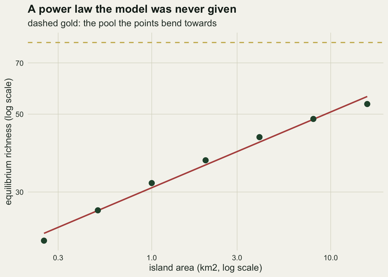
The turnover a survey reports depends on its gap
The last measurement is the one that matters for fieldwork. Turnover is almost always reported as the fraction of the first survey’s species missing from the second, and that fraction depends on how long the two surveys were apart in a way that is not proportional.
gap_grid <- c(1, 2, 5, 10, 20, 40, 80, 160)
set.seed(551)
occ_gap <- sim_island(ns_col, ns_ext, n_burn + 600, n_gap_rep)
win_gap <- (n_burn + 1):(n_burn + 601)
gap_tab <- do.call(rbind, lapply(gap_grid, function(g) {
  tf <- win_gap[win_gap + g <= max(win_gap)]
  v <- vapply(seq_len(n_gap_rep), function(r) {
    was <- occ_gap[, r, tf]; sum(was & !occ_gap[, r, tf + g]) / sum(was)
  }, 0)
  data.frame(gap = g, lost = mean(v), se = sd(v) / sqrt(n_gap_rep))
}))
gap_tab$per_year <- gap_tab$lost / gap_tab$gap
sat_ana  <- sum(ns_cf$p_pres * (1 - ns_cf$p_pres)) / sum(ns_cf$p_pres)
gap_lo   <- min(gap_grid); gap_hi <- max(gap_grid)
i_lo     <- match(gap_lo, gap_tab$gap); i_hi <- match(gap_hi, gap_tab$gap)
rate_drop <- gap_tab$per_year[i_lo] / gap_tab$per_year[i_hi]
gap_show  <- c(1, 10, 40, 160); lost_show <- gap_tab$lost[match(gap_show, gap_tab$gap)]
sat_off   <- 100 * abs(gap_tab$lost[i_hi] - sat_ana)
Across 30 islands, a gap of 1 year loses 9.1 per cent of the list; 10 years lose 43.7 per cent; 40 years lose 54.3 per cent; 160 years lose 54.6 per cent. The measured fraction stops climbing well before the gap runs out, and the longest gap lands 0.3 percentage points from the value the algebra predicts, 0.543, which is the residence weighted average probability of being absent. Beyond that ceiling the second survey is a draw from the stationary distribution that has forgotten the first, and a longer wait adds nothing. The consequence for reporting comes from dividing the measured fraction by the gap, which gives an apparent turnover rate per year. That rate falls by a factor of 27 between a gap of 1 year and a gap of 160 years, on an island where the true rate never changes. Two studies of the same island with different resurvey intervals will report different turnover rates and both will be arithmetically correct.
p_sat <- ggplot(gap_tab, aes(gap, lost)) +
  geom_hline(yintercept = sat_ana, colour = te_rust, linetype = "dashed", linewidth = 0.7) +
  geom_line(colour = te_forest, linewidth = 0.8) +
  geom_point(size = 2.6, colour = te_forest) +
  scale_x_log10() + scale_y_continuous(limits = c(0, 0.62)) +
  labs(x = "years between surveys (log scale)",
       y = "fraction of the first list missing",
       title = "Turnover saturates",
       subtitle = "dashed red: the algebraic ceiling") +
  theme_datasheet()

p_rate <- ggplot(gap_tab, aes(gap, per_year)) +
  geom_line(colour = te_gold, linewidth = 0.8) +
  geom_point(size = 2.6, colour = te_gold) +
  scale_x_log10() + scale_y_log10() +
  labs(x = "years between surveys (log scale)",
       y = "fraction divided by the gap",
       title = "The reported rate does not",
       subtitle = "one island, one rate, eight answers") +
  theme_datasheet()

p_sat + p_rate + plot_annotation(theme = theme_datasheet())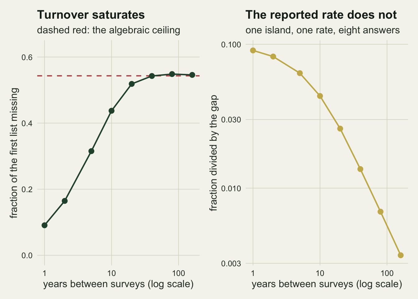
Diamond (1969) resurveyed the Channel Islands avifauna against censuses about fifty years older and read the differences as turnover at equilibrium. Lynch and Johnson (1974) went back over the same comparison and argued that much of the apparent turnover was pseudoturnover: species missed in one of the two censuses, taxonomic changes, and populations that were never resident. That dispute is about a different error from the one measured here, but they compound, and both push in the direction of reading more replacement into a pair of lists than the island performed.
What to report
Report the survey interval next to any turnover figure, and report the raw counts the fraction came from: how many species on the first list, how many of those were missing from the second, how many were new. A percentage without its interval is not comparable with anything, and the table above shows how far apart two correct percentages can be. Report gross change and net change separately as well: net change is what a richness time series shows and it is the smaller number by a wide margin; in this simulation the gross change across a decade was 6.6 times the net change, plus or minus 0.08. A monitoring programme that only publishes richness is discarding most of what it measured.
If a turnover rate per year is wanted, do not divide a long interval fraction by the interval. Fit the two state model instead: with a pair of surveys and an assumption of stationarity, the fraction lost and the fraction gained identify a residence probability and a relaxation rate, and the annual rate follows from those. Those two numbers are pool averages weighted by residence, not any one species’ rates, because the pool here is heterogeneous: the saturating ceiling above is exactly such a weighted mixture, and a species level fit needs more than one gap. That estimate at least does not change when the resurvey happens to be scheduled a decade later.
State the pool, because every quantity here is relative to a mainland species list defined in advance: turnover measured against a generously drawn pool including vagrants will be higher than turnover measured against a list of plausible residents, and the same island produces either answer. Then separate the two geographical effects if the design allows it, since richness alone would not distinguish a near small island from a far large one of matched richness while their churn differed, so a resurvey carries information a single census does not.
Honest limits
Species are independent in this model, which is the largest simplification and the one MacArthur and Wilson also made in the version everyone quotes. There is no competition, no priority effect and no facilitation, so the extinction rate of a species does not depend on which other species are present. Real turnover is partly interactive, and a model with interactions can produce the same equilibrium richness with a quite different turnover rate, so the churn numbers here should be read as what a non-interactive pool gives and not as a prediction for a particular taxon.
The rates are constant in time and the pool is fixed. Nothing in the simulation allows the mainland to change, the island to erode or emerge, or the climate to move, so the equilibrium is a genuine stationary state rather than a slowly moving target. Real islands are geologically young or old, and the general dynamic theory of island biogeography takes that ontogeny seriously; here it is absent by construction. The area to extinction link is an assumption in the same way: extinction rate was set to fall as area to a fixed power, a compressed stand-in for the chain from area to population size to extinction risk, so the species-area exponent reported above inherits whatever that choice was rather than earning it.
Detection is perfect here. Every species present at a survey date is recorded, so the entire measured turnover is real turnover, which is exactly the assumption Lynch and Johnson (1974) attacked. In the field, imperfect detection inflates apparent turnover in both directions at once, and separating it from the real thing needs repeat visits within a survey and an occupancy model, which this post does not attempt.
The single island is closed to anything but the mainland. Hanski (1998) makes the case that most fragmented systems are better read as a network in which every patch is both a source and a sink, and the metapopulation capacity tutorial computes the corresponding landscape quantity. An island near a large archipelago has a colonisation rate that depends on the states of its neighbours, and that feedback is not in the chain used here.
References
MacArthur RH, Wilson EO 1967 The Theory of Island Biogeography (ISBN 978-0-691-08836-5)
Simberloff DS, Wilson EO 1969 Ecology 50(2):278-296 (10.2307/1934856)
Simberloff DS, Wilson EO 1970 Ecology 51(5):934-937 (10.2307/1933995)
Diamond JM 1969 Proceedings of the National Academy of Sciences 64(1):57-63 (10.1073/pnas.64.1.57)
Lynch JF, Johnson NK 1974 The Condor 76(4):370-384 (10.2307/1365812)
Hanski I 1998 Nature 396(6706):41-49 (10.1038/23876)
Triantis KA, Guilhaumon F, Whittaker RJ 2012 Journal of Biogeography 39(2):215-231 (10.1111/j.1365-2699.2011.02652.x)