SLOSS and reserve configuration

Single large or several small? Simulate reserve configurations in R and measure the two properties that decide it: beta diversity and environmental correlation.

A planning authority has a hundred hectares to protect and a map with several candidate blocks on it. One block is a hundred hectares on its own. The alternative is eight blocks of twelve and a half hectares each, scattered across the same district. The total area is identical, the budget is identical, and the two options are supposed to be compared on ecological grounds. This is the SLOSS question, single large or several small, and it has been argued since the middle of the 1970s without settling.

It has not settled because it has no general answer. The comparison depends on properties of the particular system, and the useful thing an analyst can do is find out which properties, then measure them. This post builds the comparison twice, once for species richness and once for population persistence, and each time the answer turns on one quantity. For richness it is how much the species pool turns over between places. For persistence it is how strongly the environment varies in step across the district. Neither is a constant of nature; both are measurable in principle and badly measured in practice.

The persistence half of this post assumes you are comfortable with patch networks and extinction probabilities. If you are not, metapopulation capacity sets up the same kind of simulation with the emphasis on connectivity rather than on configuration. Here dispersal is switched off for most of the argument and only turned on at the end, because the cleanest version of the SLOSS question is about independent bets.

library(ggplot2)

te_pal <- list(forest = "#275139", green = "#2f8f63", sage = "#93a87f",
               clay = "#b5534e", gold = "#cda23f", line = "#dad9ca",
               ink = "#16241d", paper = "#f5f4ee")

theme_te <- function() {
  theme_minimal(base_size = 12) +
    theme(panel.grid.minor = element_blank(),
          panel.grid.major = element_line(colour = "#e7e6dc"),
          plot.background = element_rect(fill = "#f5f4ee", colour = NA),
          panel.background = element_rect(fill = "#f5f4ee", colour = NA),
          plot.title = element_text(face = "bold", colour = te_pal$ink),
          axis.title = element_text(colour = "#2c3a31"))
}

A species pool with a dial for turnover

The simulator holds three things fixed and varies one. Fixed: the total protected area, the species pool, and the total length of environmental gradient that the protected land covers. Varied: how wide a slice of the gradient each species can occupy.

Each candidate reserve is a square block. Its edge is degraded to a stated depth, so a block of area \(a\) has usable core area \((\sqrt{a} - 2d)^2\). That is the only mechanism in the richness model that penalises small blocks as such, and it is deliberately the only one, because the passive sampling argument below shows that without it there is nothing to penalise.

Blocks sit at positions along an environmental gradient running from 0 to 1. A single hundred hectare block covers a contiguous interval of the gradient; \(k\) blocks of area \(A/k\) each cover an interval proportional to their side length, and they are spread evenly across the whole gradient. The total gradient covered therefore rises with the number of blocks, which is the geometric fact the several small case rests on: the same hectares, spread out, touch more of the environment.

Species \(i\) has an optimum \(u_i\) on the gradient and a density \(\lambda_i\) at that optimum, drawn from a lognormal so that most species are rare and a few are common. Its density at gradient position \(g\) falls off as a Gaussian of width \(w\). The expected number of individuals of species \(i\) in a block is \(\lambda_i\) times the block’s core area times the average of that Gaussian over the block’s gradient interval, and the species is present with probability \(1 - e^{-N}\), which is Poisson placement. The width \(w\) is the dial: wide niches mean every block draws from the same set of species and differs only by area, narrow niches mean blocks in different places hold different species.

set.seed(20260719)

n_species <- 300
area_total <- 100      # hectares of protected land, fixed across configurations
edge_depth <- 0.5      # degraded edge depth, in units of 100 m
grad_span  <- 0.3      # gradient covered by the single 100 ha block
config_k   <- c(1, 2, 4, 8)

core_area <- function(a, d = edge_depth) pmax(sqrt(a) - 2 * d, 0)^2

patch_layout <- function(k, d = edge_depth) {
  a <- area_total / k
  data.frame(area = a, core = core_area(a, d),
             centre = (2 * seq_len(k) - 1) / (2 * k),
             halfwidth = 0.5 * grad_span * sqrt(a / area_total))
}

density_opt <- exp(rnorm(n_species, log(0.01), 2))
niche_opt   <- runif(n_species)

expected_n <- function(k, w, d = edge_depth, ngrid = 41) {
  pl <- patch_layout(k, d)
  out <- matrix(0, nrow = k, ncol = n_species)
  for (j in seq_len(k)) {
    gg <- seq(pl$centre[j] - pl$halfwidth[j], pl$centre[j] + pl$halfwidth[j],
              length.out = ngrid)
    out[j, ] <- density_opt * pl$core[j] *
      colMeans(exp(-outer(gg, niche_opt, "-")^2 / (2 * w^2)))
  }
  out
}

occ_prob <- function(k, w, d = edge_depth) 1 - exp(-expected_n(k, w, d))

layout_tab <- do.call(rbind, lapply(config_k, function(k) {
  pl <- patch_layout(k)
  data.frame(patches = k, patch_area = pl$area[1], core_per_patch = pl$core[1],
             core_total = sum(pl$core), gradient_covered = sum(2 * pl$halfwidth))
}))
print(round(layout_tab, 3))

  patches patch_area core_per_patch core_total gradient_covered
1       1      100.0         81.000     81.000            0.300
2       2       50.0         36.858     73.716            0.424
3       4       25.0         16.000     64.000            0.600
4       8       12.5          6.429     51.431            0.849

round(c(species_in_pool = n_species, total_area_ha = area_total,
        edge_depth_m = 100 * edge_depth), 3)

species_in_pool   total_area_ha    edge_depth_m 
            300             100              50 

The geometry is already an argument. One block of 100 hectares keeps 81 hectares of core and touches 0.3 of the gradient. Eight blocks of 12.5 hectares keep 6.429 hectares of core each, so 51.431 in total, and touch 0.849 of it. Splitting the estate throws away interior and buys nearly three times as much environmental coverage. Everything below is a fight between those two effects.

To measure how nested the resulting assemblages are, use NODF, the nestedness metric based on overlap and decreasing fill. For a pair of rows in a block by species incidence matrix, if one row has more species than the other, the pair contributes the percentage of the poorer row’s species that also occur in the richer one; pairs with equal totals contribute nothing. The same is done for columns, and the average over all pairs is the index. A metric is worth nothing until it has been run on cases whose answer is known, so run it on a perfectly nested triangular matrix and on a set of blocks with no species in common.

nodf <- function(M) {
  M <- M[, colSums(M) > 0, drop = FALSE]
  M <- M[rowSums(M) > 0, , drop = FALSE]
  pair_part <- function(tot, ov) {
    cc <- 100 * ov / outer(tot, tot, pmin)
    cc[outer(tot, tot, "==")] <- 0
    sum(cc[upper.tri(cc)])
  }
  nr <- nrow(M); nc <- ncol(M)
  (pair_part(rowSums(M), M %*% t(M)) + pair_part(colSums(M), t(M) %*% M)) /
    (nr * (nr - 1) / 2 + nc * (nc - 1) / 2)
}

perfect_nested <- matrix(0, 8, 8)
for (i in 1:8) perfect_nested[i, seq_len(9 - i)] <- 1
perfect_turnover <- matrix(0, 3, 12)
perfect_turnover[1, 1:6] <- 1; perfect_turnover[2, 7:10] <- 1
perfect_turnover[3, 11:12] <- 1
round(c(nodf_perfectly_nested = nodf(perfect_nested),
        nodf_perfectly_disjoint = nodf(perfect_turnover)), 3)

  nodf_perfectly_nested nodf_perfectly_disjoint 
                    100                       0 

The triangular matrix returns 100 and the disjoint one returns 0, so the index runs the right way and the two ends mean what they should.

Richness at a fixed total area

The incidence matrix that goes into NODF is the survey of all fifteen candidate blocks: the single large one, the two halves, the four quarters and the eight eighths. That is a matrix a planner could actually assemble, and it spans the range of block sizes under discussion, which NODF needs in order to have a fill gradient to work on. Total richness of a configuration is the number of species present in at least one of its blocks, averaged over replicate assemblages.

n_assem <- 100

assemble <- function(w, nrep = n_assem) {
  probs <- lapply(config_k, function(k) occ_prob(k, w))
  stack <- do.call(rbind, probs)
  rich <- matrix(0, nrep, length(config_k))
  nod <- numeric(nrep)
  for (i in seq_len(nrep)) {
    draw <- matrix(rbinom(length(stack), 1, stack), nrow(stack), ncol(stack))
    rows <- rep(config_k, config_k)
    for (j in seq_along(config_k)) {
      sub <- draw[rows == config_k[j], , drop = FALSE]
      rich[i, j] <- sum(colSums(sub) > 0)
    }
    nod[i] <- nodf(draw)
  }
  c(nodf = mean(nod), setNames(colMeans(rich), paste0("k", config_k)))
}

w_nested <- 1.5
w_turnover <- 0.06
res_nested <- assemble(w_nested)
res_turnover <- assemble(w_turnover)
print(round(rbind(nested = res_nested, turnover = res_turnover), 2))

          nodf     k1     k2     k4     k8
nested   64.48 171.57 166.41 159.51 147.21
turnover 22.32  50.58  71.90  71.52  63.31

round(c(niche_width_nested = w_nested, niche_width_turnover = w_turnover,
        assemblage_replicates = n_assem), 3)

   niche_width_nested  niche_width_turnover assemblage_replicates 
                 1.50                  0.06                100.00 

pool_levels <- c(sprintf("Nested pool, NODF %.1f", res_nested["nodf"]),
                 sprintf("Turnover pool, NODF %.1f", res_turnover["nodf"]))
rich_long <- rbind(
  data.frame(patches = config_k, richness = as.numeric(res_nested[-1]),
             base = as.numeric(res_nested["k1"]), pool = pool_levels[1]),
  data.frame(patches = config_k, richness = as.numeric(res_turnover[-1]),
             base = as.numeric(res_turnover["k1"]), pool = pool_levels[2]))
rich_long$pool <- factor(rich_long$pool, levels = pool_levels)
side_levels <- c("single large block", "split at least equal", "single large ahead")
rich_long$side <- factor(ifelse(
  rich_long$patches == 1, side_levels[1],
  ifelse(rich_long$richness >= rich_long$base, side_levels[2], side_levels[3])),
  levels = side_levels)
base_line <- unique(rich_long[, c("pool", "base")])

ggplot(rich_long, aes(factor(patches), richness, fill = side)) +
  geom_col(width = 0.68) +
  geom_hline(data = base_line, aes(yintercept = base), colour = te_pal$ink,
             linetype = "22", linewidth = 0.6) +
  facet_wrap(~pool, scales = "free_y") +
  scale_fill_manual(values = setNames(c(te_pal$forest, te_pal$green, te_pal$sage),
                                      side_levels), name = NULL) +
  labs(x = "Number of blocks the hundred hectares is split into",
       y = "Total species richness",
       title = "Splitting the same hectares helps only when the pool turns over") +
  theme_te() +
  theme(legend.position = "top",
        strip.text = element_text(colour = te_pal$ink, face = "bold"))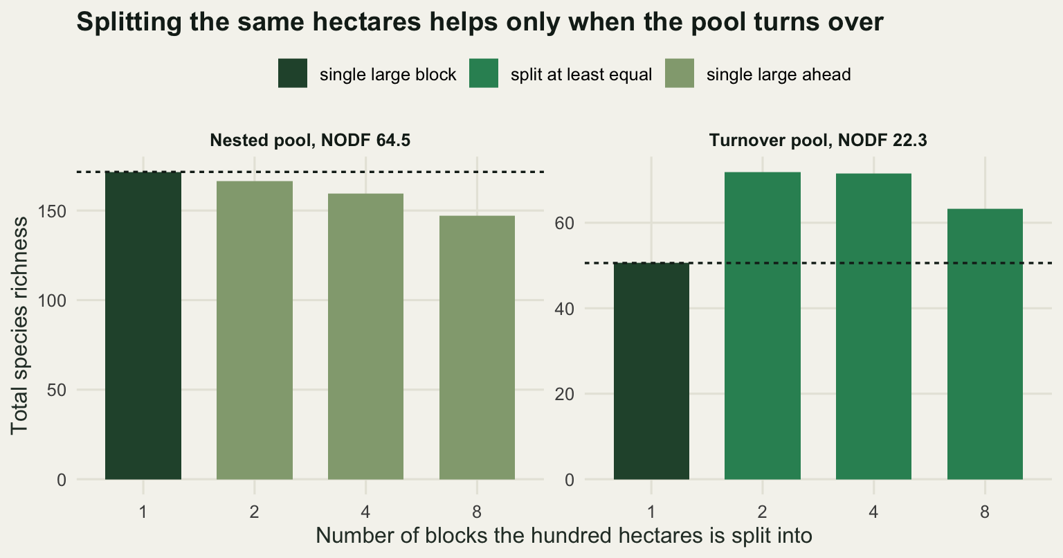

Figure 1: Total species richness of four reserve configurations holding the same hundred hectares, under a strongly nested species pool and a strongly turnover dominated one. The dashed line in each panel is the single large block.

Under wide niches the assemblages are strongly nested, NODF 64.48, and the ranking is the one the old reserve design rules assert: 171.57 species in the single large block, 166.41 across two, 159.51 across four and 147.21 across eight. Splitting the estate eight ways takes the total from 171.57 down to 147.21. Under narrow niches, NODF 22.32, the ranking reverses and the margin is larger in relative terms: 50.58 species in the single large block against 71.90 across two, 71.52 across four and 63.31 across eight. The single large block is now the worst of the four options by a clear margin.

Two details in those numbers matter more than the headline. The first is that several small is not monotone in the number of blocks. Under the turnover pool, two and four blocks are indistinguishable and eight is clearly worse than either, because by then each block is small enough that the edge penalty and the loss of rare species to sampling outrun the gain in gradient coverage. There is an interior optimum, and “several” is not a synonym for “as many as possible”.

The second is where the one large advantage comes from in the nested case. It is not from sampling. Set the edge depth to zero and repeat.

rich_expected <- function(k, w, d) {
  p <- occ_prob(k, w, d)
  sum(1 - apply(1 - p, 2, prod))
}
no_edge <- sapply(config_k, function(k) rich_expected(k, w_nested, 0))
with_edge <- sapply(config_k, function(k) rich_expected(k, w_nested, edge_depth))
print(round(rbind(no_edge = setNames(no_edge, paste0("k", config_k)),
                  with_edge = with_edge), 3))

               k1      k2      k4      k8
no_edge   182.701 182.072 181.929 181.899
with_edge 172.076 166.644 159.287 148.105

round(c(no_edge_spread = max(no_edge) - min(no_edge),
        with_edge_spread = max(with_edge) - min(with_edge)), 3)

  no_edge_spread with_edge_spread 
           0.802           23.970 

With no edge effect and a nested pool, the four configurations return 182.701, 182.072, 181.929 and 181.899 species, a spread of 0.802 species across an eightfold split. That is a tie, and it is not an accident of the parameters. When species are placed at random and detected in proportion to the area sampled, the probability that a species misses all of \(k\) blocks of area \(A/k\) is the same as the probability that it misses one block of area \(A\), so the two configurations have the same expected richness exactly. Random placement predicts a draw. Restore the 50 m edge and the spread across the same four configurations jumps to 23.970 species. The whole of the one large advantage in the nested case is the edge penalty, which is a statement about the biology of a particular species pool and not about area at all.

Where the richness answer flips

Sweeping the niche width across three orders of magnitude gives, for each pool, a nestedness value and a richness for each configuration. The crossover is the nestedness at which the difference between a configuration and the single large block changes sign.

n_sweep <- 60
w_grid <- exp(seq(log(0.015), log(3), length.out = 16))
sweep_tab <- as.data.frame(t(sapply(w_grid, function(w) c(w = w, assemble(w, n_sweep)))))
sweep_tab$d2 <- sweep_tab$k2 - sweep_tab$k1
sweep_tab$d4 <- sweep_tab$k4 - sweep_tab$k1
sweep_tab$d8 <- sweep_tab$k8 - sweep_tab$k1
print(round(sweep_tab, 2))

      w  nodf     k1     k2     k4     k8    d2     d4     d8
1  0.01 10.99  22.72  24.45  27.83  25.20  1.73   5.12   2.48
2  0.02 12.63  27.20  31.32  36.52  32.97  4.12   9.32   5.77
3  0.03 14.91  33.55  40.88  47.80  41.58  7.33  14.25   8.03
4  0.04 18.09  40.93  55.77  60.22  51.60 14.83  19.28  10.67
5  0.06 22.86  51.42  74.08  73.18  63.05 22.67  21.77  11.63
6  0.09 27.97  67.03  91.05  86.38  76.98 24.02  19.35   9.95
7  0.12 36.15  92.78 109.68 100.60  88.85 16.90   7.82  -3.93
8  0.18 45.52 122.20 122.17 114.97 102.57 -0.03  -7.23 -19.63
9  0.25 53.43 143.92 134.87 126.43 116.40 -9.05 -17.48 -27.52
10 0.36 59.05 157.48 147.85 139.98 129.02 -9.63 -17.50 -28.47
11 0.51 62.25 163.55 156.42 148.30 136.70 -7.13 -15.25 -26.85
12 0.73 63.53 169.58 162.82 153.82 142.70 -6.77 -15.77 -26.88
13 1.04 64.13 171.85 163.53 156.93 145.60 -8.32 -14.92 -26.25
14 1.48 64.23 171.73 166.23 158.10 148.73 -5.50 -13.63 -23.00
15 2.11 64.98 174.15 168.57 159.87 147.77 -5.58 -14.28 -26.38
16 3.00 64.52 172.90 167.58 160.43 149.53 -5.32 -12.47 -23.37

round(c(sweep_points = length(w_grid), sweep_replicates = n_sweep), 3)

    sweep_points sweep_replicates 
              16               60 

cross_nodf <- function(dv) {
  top <- which.max(dv)
  j <- top - 1 + which(dv[top:length(dv)] < 0)[1]
  approx(dv[c(j - 1, j)], sweep_tab$nodf[c(j - 1, j)], 0)$y
}
nodf_cross <- c(two = cross_nodf(sweep_tab$d2), four = cross_nodf(sweep_tab$d4),
                eight = cross_nodf(sweep_tab$d8))
print(round(nodf_cross, 2))

  two  four eight 
45.51 41.02 33.83 

Four blocks beat one block whenever NODF is below 39.89. Two blocks hold on until 46.69 and eight blocks give up at 33.89, so the more finely the estate is divided, the more turnover the pool has to show before the division pays. Nestedness above 46.69 in this system means one large wins whatever the split; below 33.89 several small wins whatever the split; between those two values the answer depends on how many blocks, which is the interesting region and also the one no rule of thumb covers.

The sweep contains a result I did not expect and have kept. The advantage of several small is not largest at the most turnover dominated end of the dial. It peaks in the middle. At NODF 22.71 the four block configuration is 20.88 species ahead; push the pool further towards turnover, to NODF 10.99, and the lead falls to 5.12 species. The reason is that once niches are narrower than the gradient interval a single block covers, both configurations are sampling the same total length of gradient, and the geometric advantage of spreading out disappears while the edge penalty stays. Extreme turnover is not the friend of several small; moderate turnover is.

What a species-area relationship can and cannot settle

The oldest way to argue SLOSS is to write down a power law species-area relationship, \(S = cA^{z}\), and compare \(c A^{z}\) against the total for \(k\) blocks of area \(A/k\). If the blocks share no species, that total is \(k \, c (A/k)^{z} = cA^{z} k^{1-z}\), and the ratio of several small to one large is \(k^{1-z}\). Since \(z\) in published species-area relationships sits between about 0.15 and 0.35, that ratio is well above one and several small wins by a wide margin. The calculation is done in a line and it settles nothing, because the sharing assumption is doing all the work.

Give the blocks an overlap. Let each of the \(k\) blocks hold \(S_s = c(A/k)^z\) species drawn at random from a regional pool of \(S_R\) species, and let \(o = S_s / S_R\) be the expected proportion of one block’s species that also occur in any other given block. The expected number of distinct species across the network is then \(S_R(1 - (1 - o)^k) = (S_s/o)(1 - (1-o)^k)\), and setting that equal to \(cA^z\) gives a break-even exponent that no longer depends on \(c\) or \(A\):

\[z^{*} = \frac{\log\!\left[(1 - (1-o)^{k}) / o\right]}{\log k}\]

sar_c <- 20
k_sar <- 4
ss_over_ol <- function(z, k, o) {
  s_small <- sar_c * (area_total / k)^z
  tot <- if (o <= 0) k * s_small else (s_small / o) * (1 - (1 - o)^k)
  tot / (sar_c * area_total^z)
}
z_star <- function(k, o) if (o <= 0) 1 else log((1 - (1 - o)^k) / o) / log(k)

z_show <- c(0.15, 0.25, 0.35, 0.45, 0.55)
sar_tab <- data.frame(
  z = z_show,
  one_large = sar_c * area_total^z_show,
  four_independent = sapply(z_show, function(z) sar_c * area_total^z * ss_over_ol(z, k_sar, 0)),
  four_half_shared = sapply(z_show, function(z) sar_c * area_total^z * ss_over_ol(z, k_sar, 0.5)))
print(round(sar_tab, 2))

     z one_large four_independent four_half_shared
1 0.15     39.91           129.65            60.77
2 0.25     63.25           178.89            83.85
3 0.35    100.24           246.81           115.69
4 0.45    158.87           340.54           159.63
5 0.55    251.79           469.85           220.24

round(c(sar_c = sar_c, patches = k_sar, overlap = 0.5,
        z_equal_independent = z_star(k_sar, 0),
        z_equal_half_shared = z_star(k_sar, 0.5),
        z_equal_quarter_shared = z_star(k_sar, 0.25),
        z_equal_three_quarter_shared = z_star(k_sar, 0.75)), 4)

                       sar_c                      patches 
                     20.0000                       4.0000 
                     overlap          z_equal_independent 
                      0.5000                       1.0000 
         z_equal_half_shared       z_equal_quarter_shared 
                      0.4534                       0.7256 
z_equal_three_quarter_shared 
                      0.2047 

z_seq <- seq(0.05, 0.85, length.out = 160)
ov_show <- c(0, 0.25, 0.5, 0.75)
ov_lab <- sprintf("%.0f per cent shared", 100 * ov_show)
sar_long <- do.call(rbind, lapply(seq_along(ov_show), function(i) data.frame(
  z = z_seq, overlap = ov_lab[i],
  gain = sar_c * area_total^z_seq * (ss_over_ol(z_seq, k_sar, ov_show[i]) - 1))))
sar_long$overlap <- factor(sar_long$overlap, levels = ov_lab)
zs <- sapply(ov_show, function(o) z_star(k_sar, o))
marks <- data.frame(z = zs, gain = 0, overlap = factor(ov_lab, levels = ov_lab))
marks <- marks[marks$z <= max(z_seq), ]

ggplot(sar_long, aes(z, gain, colour = overlap)) +
  geom_hline(yintercept = 0, colour = te_pal$ink, linewidth = 0.6) +
  geom_line(linewidth = 0.9) +
  geom_point(data = marks, size = 3) +
  scale_colour_manual(values = c(te_pal$forest, te_pal$green, te_pal$gold,
                                 te_pal$clay), name = NULL) +
  coord_cartesian(ylim = c(-120, 260)) +
  labs(x = "Species-area exponent z",
       y = "Four blocks minus one block, species",
       title = "A species-area exponent alone cannot settle the question") +
  theme_te() +
  theme(legend.position = "top")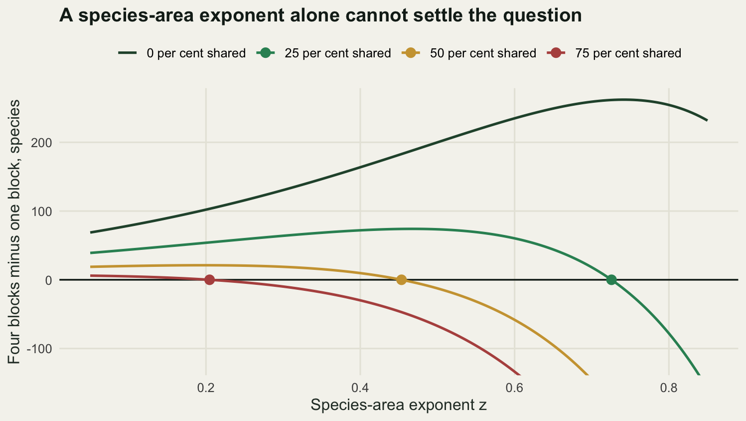

Figure 2: Species gained or lost by splitting a hundred hectares into four blocks, as a function of the species-area exponent, for four levels of species sharing between blocks. The horizontal line is equality and the dots mark the break-even exponent.

With independent blocks the break-even exponent is 1, which is to say there is no break-even inside the range any real species-area curve occupies. At \(z = 0.25\) with \(c = 20\) and a hundred hectares, one large block is predicted to hold 63.25 species and four independent blocks 178.89. Let half of each block’s species also occur in any other block and the same four blocks are predicted to hold 83.85, still ahead but by a far smaller margin, and the break-even exponent drops from 1 to 0.4534. At a quarter shared it is 0.7256 and at three quarters shared it is 0.2047, which is inside the range of exponents people actually fit.

The exponent is easy to estimate and it is the wrong number to estimate. It is a within-network description of how richness accumulates with area, and the SLOSS comparison needs a between-block description of how much the blocks duplicate each other. Reporting \(z\) without the overlap is reporting the half of the calculation that cannot change the answer.

Persistence with correlated environments

Richness counts species on a map at one moment. The other half of a reserve decision is whether anything is still there in a century. Take one species, give it a total carrying capacity proportional to the total protected area, and split that capacity between the blocks. Each subpopulation grows by a Ricker rule with demographic stochasticity from Poisson offspring numbers and environmental stochasticity from an annual lognormal multiplier on the growth rate. Between blocks, the environmental deviations are correlated with correlation \(\rho\): each year draws one shared deviate and one independent deviate per block, weighted \(\sqrt{\rho}\) and \(\sqrt{1-\rho}\). Dispersal is zero for now, so the blocks are separate bets on the same species. The configuration persists if at least one subpopulation is alive at the horizon.

The whole projection is one matrix of replicates by blocks stepped forward year by year, which is why a hundred years of several thousand replicates costs a second rather than a minute.

r_max <- 0.15
k_total <- 400
sig_env <- 0.4
horizon <- 100

net_run <- function(k, rho, disp = 0, nrep = 3000, keep = FALSE) {
  kp <- k_total / k
  n <- matrix(kp, nrep, k)
  occ <- if (keep) array(FALSE, c(nrep, k, horizon)) else NULL
  for (t in seq_len(horizon)) {
    e <- sqrt(rho) * rnorm(nrep) + sqrt(1 - rho) * matrix(rnorm(nrep * k), nrep, k)
    mu <- n * exp(r_max * (1 - n / kp) + sig_env * e - sig_env^2 / 2)
    n <- matrix(rpois(nrep * k, mu), nrep, k)
    if (disp > 0 && k > 1) {
      em <- matrix(rbinom(nrep * k, n, disp), nrep, k)
      n <- n - em
      rem <- rowSums(em)
      for (j in seq_len(k - 1)) {
        got <- rbinom(nrep, rem, 1 / (k - j + 1))
        n[, j] <- n[, j] + got
        rem <- rem - got
      }
      n[, k] <- n[, k] + rem
    }
    if (keep) occ[, , t] <- n > 0
  }
  if (keep) list(persist = mean(rowSums(n) > 0), occ = occ) else mean(rowSums(n) > 0)
}

set.seed(4102)
n_rep_main <- 3000
rho_show <- c(0, 0.5, 1)
p_large <- net_run(1, 0, nrep = 8000)
pers_tab <- do.call(rbind, lapply(rho_show, function(rr)
  data.frame(rho = rr, patches = config_k,
             persist = c(p_large, sapply(config_k[-1], function(k)
               net_run(k, rr, nrep = n_rep_main))))))
print(round(reshape(pers_tab, idvar = "patches", timevar = "rho", direction = "wide"), 4))

  patches persist.0 persist.0.5 persist.1
1       1    0.8058      0.8058    0.8058
2       2    0.8803      0.8433    0.7947
3       4    0.9037      0.8330    0.7397
4       8    0.8450      0.7357    0.6273

round(c(horizon_years = horizon, replicates = n_rep_main, total_K = k_total,
        r_max = r_max, sigma_env = sig_env, one_large_persistence = p_large), 4)

        horizon_years            replicates               total_K 
             100.0000             3000.0000              400.0000 
                r_max             sigma_env one_large_persistence 
               0.1500                0.4000                0.8058 

A single population at a carrying capacity of 400, growing at 0.15 with an environmental standard deviation of 0.4, survives a hundred years in 0.8058 of replicates. It has no correlation to have, so its row of the table is one number repeated.

When the blocks are environmentally independent, splitting is a portfolio and the portfolio wins: 0.8803 for two blocks, 0.9037 for four, 0.8450 for eight. When the blocks share their bad years completely, splitting is a pure cost and the ranking inverts: 0.7947, 0.7397 and 0.6273. At a correlation of one half the two block network is still ahead at 0.8433, the four block network is ahead by a hair at 0.8330, and the eight block network has already fallen behind at 0.7357.

Eight blocks is worse than four at every correlation including zero, which is the same interior optimum the richness half of the post found, arriving by an unrelated route. Independence is worth something, but each independent bet has to be large enough to be worth placing, and at an eighth of the total carrying capacity it is not.

The crossover correlation

The number a planner needs is the correlation at which the ranking flips. Run the four block network across a grid of correlations, subtract the single large block’s probability, fit a quadratic to the difference to average out the Monte Carlo noise, and solve for the root.

set.seed(707)
n_rep_cross <- 4000
rho_grid <- seq(0, 1, by = 0.125)

cross_rho <- function(disp, nrep = n_rep_cross) {
  pv <- sapply(rho_grid, function(rr) net_run(4, rr, disp = disp, nrep = nrep))
  dv <- pv - p_large
  fit <- lm(dv ~ rho_grid + I(rho_grid^2))
  cf <- coef(fit)
  rts <- if (abs(cf[3]) < 1e-8) -cf[1] / cf[2] else
    Re(polyroot(c(cf[1], cf[2], cf[3])))
  rts <- rts[is.finite(rts)]
  inside <- rts[rts >= 0 & rts <= 1.6]
  list(p = pv, d = dv, cross = if (length(inside)) min(inside) else NA)
}

cr0 <- cross_rho(0)
round(c(crossover_replicates = n_rep_cross), 0)

crossover_replicates 
                4000 

round(c(mc_se_of_difference = sqrt(2 * 0.85 * 0.15 / n_rep_main)), 4)

mc_se_of_difference 
             0.0092 

print(round(data.frame(rho = rho_grid, four_small = cr0$p, difference = cr0$d), 4))

    rho four_small difference
1 0.000     0.9002     0.0945
2 0.125     0.8900     0.0843
3 0.250     0.8662     0.0605
4 0.375     0.8478     0.0420
5 0.500     0.8348     0.0290
6 0.625     0.8130     0.0072
7 0.750     0.7808    -0.0250
8 0.875     0.7530    -0.0527
9 1.000     0.7170    -0.0887

round(c(crossover_rho_four_patches = cr0$cross), 4)

crossover_rho_four_patches 
                    0.6367 

set.seed(88)
pers_cross <- sapply(config_k, function(k) net_run(k, cr0$cross, nrep = n_rep_main))
round(setNames(pers_cross, paste0("k", config_k)), 4)

    k1     k2     k4     k8 
0.8050 0.8373 0.8113 0.7190 

rho_levels <- sort(unique(c(rho_show, round(cr0$cross, 3))))
pers_fig <- rbind(pers_tab,
                  data.frame(rho = round(cr0$cross, 3), patches = config_k,
                             persist = pers_cross))
pers_fig$lab <- factor(sprintf("rho = %.3f", pers_fig$rho),
                       levels = sprintf("rho = %.3f", rho_levels))

ggplot(pers_fig, aes(patches, persist, colour = lab)) +
  geom_hline(yintercept = p_large, colour = te_pal$ink, linetype = "22",
             linewidth = 0.6) +
  geom_line(linewidth = 0.9) +
  geom_point(size = 2.4) +
  scale_x_continuous(trans = "log2", breaks = config_k) +
  scale_colour_manual(values = c(te_pal$forest, te_pal$green, te_pal$gold,
                                 te_pal$clay), name = NULL) +
  labs(x = "Number of blocks the same carrying capacity is split between",
       y = "Probability at least one subpopulation persists",
       title = "Several small patches win until the blocks share their bad years") +
  theme_te() +
  theme(legend.position = "top")

Figure 3: Probability that at least one subpopulation survives a hundred years, against the number of blocks the same carrying capacity is split between, at four levels of environmental correlation between blocks. The dashed line is the single large block.

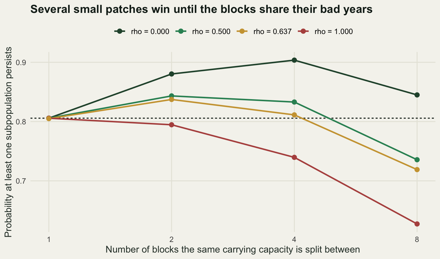
The crossover is at a correlation of 0.6367. That is the central number of the post. Below it, splitting the estate four ways raises the hundred year persistence probability; above it, splitting lowers it. Rerunning all four configurations at exactly that correlation gives 0.8050 for one block and 0.8113 for four, a gap smaller than the Monte Carlo standard error of 0.0092 on the difference, so the two are tied to within the noise, which is what a crossover should look like.

The correlation is high. Environmental deviations would have to agree between blocks better than two thirds of the way to lockstep before the single large block becomes the safer option for this species. Blocks scattered across a district, in different catchments or on different soils, are usually well below that; blocks a few kilometres apart in one valley, exposed to the same drought and the same late frost, are usually above it. The SLOSS answer for persistence is a claim about the spatial scale of environmental variation relative to the spacing of the reserves, and nothing else in the model competes with it for importance.

Dispersal moves the crossover

Turning dispersal on changes the question from a portfolio of independent bets to a network that can repair itself. Each year a fraction \(m\) of individuals leaves its block and settles in a block chosen at random from the \(k\), so a share of the emigrants comes home. Emigration is binomial and the redistribution is an exact multinomial split, done as a chain of conditional binomials so everything stays integer and demographic stochasticity is not quietly smoothed away.

set.seed(2211)
disp_rates <- c(0, 0.001, 0.01, 0.05)
disp_runs <- c(list(cr0), lapply(disp_rates[-1], function(d) cross_rho(d)))
disp_tab <- do.call(rbind, lapply(seq_along(disp_rates), function(i)
  data.frame(disp = disp_rates[i], rho = rho_grid, persist = disp_runs[[i]]$p,
             difference = disp_runs[[i]]$d)))
disp_cross <- sapply(disp_runs, function(z) z$cross)
names(disp_cross) <- paste0("m", disp_rates)
print(round(disp_cross, 4))

    m0 m0.001  m0.01  m0.05 
0.6367 0.7023 0.8054 0.9089 

print(round(reshape(disp_tab[, c("disp", "rho", "persist")], idvar = "rho",
                    timevar = "disp", direction = "wide"), 4))

    rho persist.0 persist.0.001 persist.0.01 persist.0.05
1 0.000    0.9002        0.9148       0.9725       0.9952
2 0.125    0.8900        0.8968       0.9592       0.9848
3 0.250    0.8662        0.8765       0.9372       0.9730
4 0.375    0.8478        0.8642       0.9152       0.9545
5 0.500    0.8348        0.8485       0.8752       0.9278
6 0.625    0.8130        0.8170       0.8505       0.8948
7 0.750    0.7808        0.7960       0.8302       0.8572
8 0.875    0.7530        0.7730       0.7852       0.8160
9 1.000    0.7170        0.7395       0.7445       0.7735

disp_lab <- sprintf("m = %.3f", disp_rates)
disp_tab$lab <- factor(sprintf("m = %.3f", disp_tab$disp), levels = disp_lab)
cross_pts <- data.frame(rho = as.numeric(disp_cross), difference = 0,
                        lab = factor(disp_lab, levels = disp_lab))

ggplot(disp_tab, aes(rho, difference, colour = lab)) +
  geom_hline(yintercept = 0, colour = te_pal$ink, linewidth = 0.6) +
  geom_line(linewidth = 0.9) +
  geom_point(size = 1.8) +
  geom_point(data = cross_pts, size = 3.4, shape = 18) +
  scale_colour_manual(values = c(te_pal$forest, te_pal$green, te_pal$gold,
                                 te_pal$clay), name = NULL) +
  labs(x = "Environmental correlation between blocks",
       y = "Four blocks minus one block, persistence probability",
       title = "Dispersal widens the range in which several small patches win") +
  theme_te() +
  theme(legend.position = "top")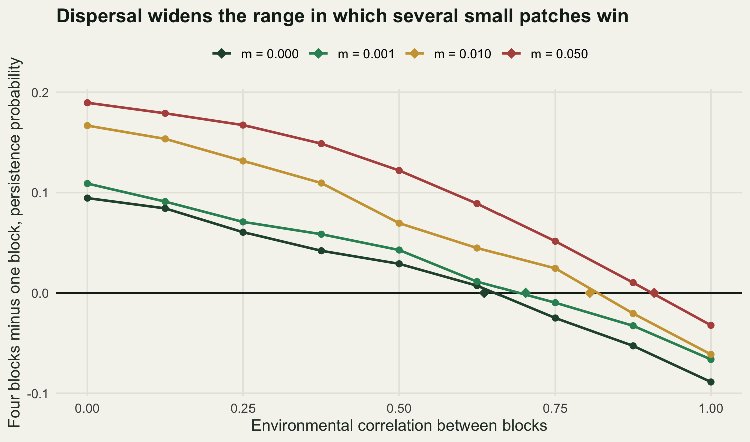

Figure 4: Persistence advantage of four blocks over one, against environmental correlation, at four dispersal rates. The horizontal line is equality and the dots on it are the crossover correlations.

The crossover moves from 0.6367 with no dispersal to 0.7023 at a rate of one in a thousand individuals a year, 0.8054 at one in a hundred, and 0.9089 at one in twenty. At a correlation of one half, the four block network persists in 0.8348 of replicates with no dispersal, 0.8485 at the lowest rate, and 0.9278 at the highest. The lowest rate barely moves anything; the highest turns a configuration that was two thirds of the way to losing into one that is comfortably ahead.

The mechanism is recolonisation, and it can be measured directly rather than asserted. Record the occupancy of every block in every year, find every block year in which a block was empty while at least one other block was occupied, and count how often that block was occupied again within ten years.

set.seed(5150)
window <- 10
recol_prob <- function(disp, rho = 0.5, nrep = 1500) {
  z <- net_run(4, rho, disp = disp, nrep = nrep, keep = TRUE)
  occ <- z$occ
  empty <- 0; refilled <- 0
  for (t in seq_len(horizon - window)) {
    now <- occ[, , t]
    others <- rowSums(now) - now
    cand <- (!now) & (others > 0)
    if (!any(cand)) next
    fut <- apply(occ[, , (t + 1):(t + window), drop = FALSE], c(1, 2), any)
    empty <- empty + sum(cand)
    refilled <- refilled + sum(cand & fut)
  }
  c(patch_years_empty = empty, recolonised = refilled, prob = refilled / empty)
}
rec_low <- recol_prob(0.001)
rec_high <- recol_prob(0.05)
print(round(rbind(low_dispersal = rec_low, high_dispersal = rec_high), 4))

               patch_years_empty recolonised  prob
low_dispersal              94802       17353 0.183
high_dispersal              9705        7308 0.753

round(c(recolonisation_window_years = window), 3)

recolonisation_window_years 
                         10 

At the lowest dispersal rate an empty block with an occupied neighbour is refilled within ten years in 0.183 of cases, from 94802 empty block years. At the highest rate the figure is 0.753, from 9705 empty block years. The second number is smaller because the same dispersal that refills blocks also stops them emptying in the first place, and that is the whole rescue effect in two counts: an order of magnitude fewer local extinctions, and four times the chance of undoing the ones that happen.

Dispersal does not rewrite the ranking, though. Every line in the figure still slopes down and still ends below zero. Even at one in twenty individuals moving each year, a set of blocks whose environments move in perfect lockstep is worse than one block of the same total capacity, because dispersal cannot import good years from a block that is having the same bad year.

What has to be known before the recommendation

The two answers rest on two quantities. The richness answer rests on how nested the pool is, and the persistence answer rests on how correlated the environments are. Both are hard to measure in the field: nestedness needs comparable inventories of many blocks spanning a range of sizes, and environmental correlation needs long parallel series from every block, which is exactly the data a new reserve network does not have. So the honest thing to do is price the error.

mis_rho <- 0.2
rho_lo <- max(cr0$cross - mis_rho, 0)
rho_hi <- min(cr0$cross + mis_rho, 1)
set.seed(1234)
p_lo <- net_run(4, rho_lo, nrep = 6000)
p_hi <- net_run(4, rho_hi, nrep = 6000)
round(c(rho_low = rho_lo, rho_high = rho_hi,
        persist_low = p_lo, persist_high = p_hi,
        diff_low = p_lo - p_large, diff_high = p_hi - p_large,
        swing = (p_lo - p_large) - (p_hi - p_large)), 4)

     rho_low     rho_high  persist_low persist_high     diff_low    diff_high 
      0.4367       0.8367       0.8335       0.7727       0.0278      -0.0331 
       swing 
      0.0608 

mis_nodf <- 20
nodf_lo <- nodf_cross["four"] - mis_nodf
nodf_hi <- nodf_cross["four"] + mis_nodf
d_at <- function(x) approx(sweep_tab$nodf, sweep_tab$d4, x)$y
round(c(nodf_crossing = as.numeric(nodf_cross["four"]),
        nodf_low = as.numeric(nodf_lo), nodf_high = as.numeric(nodf_hi),
        richness_diff_low = as.numeric(d_at(nodf_lo)),
        richness_diff_high = as.numeric(d_at(nodf_hi)),
        richness_swing = as.numeric(d_at(nodf_lo) - d_at(nodf_hi)),
        rho_error = mis_rho, nodf_error = mis_nodf), 3)

     nodf_crossing           nodf_low          nodf_high  richness_diff_low 
            41.018             21.018             61.018             20.808 
richness_diff_high     richness_swing          rho_error         nodf_error 
           -16.118             36.926              0.200             20.000 

Suppose the correlation is estimated at the crossover value and the estimate is wrong by 0.2, which for a correlation coefficient from a short series is an ordinary error. At 0.4367 the four block network persists in 0.8335 of replicates, 0.0278 above the single large block. At 0.8367 it persists in 0.7727, 0.0331 below. The recommendation is not merely uncertain across that band, it reverses, and the swing in the quantity being recommended on is 0.0608 in probability of persistence, which is larger than most of the differences the model produces anywhere.

The richness side behaves the same way and worse. Take an error of 20 NODF units, which is the same fifth of the metric’s range as 0.2 is of a correlation. The crossing for four blocks sits at 39.894. At 19.894 the four block configuration is 19.549 species ahead; at 59.894 it is 18.516 species behind. A swing of 38.065 species, on a pool whose single large block holds 171.57 species at its richest, from an error in a metric that most inventories are not designed to estimate at all.

That is the honest limit and it should be read as an instruction rather than a caveat. A SLOSS recommendation is not a general ecological principle applied to a site. It is a claim that two specific numbers, the nestedness of the pool and the environmental correlation between the candidate blocks, fall on one side of two thresholds. Anyone who makes the recommendation without those two numbers is asserting them silently, and the arithmetic above says the assertion is worth more than everything else in the analysis put together. When neither number is known, the defensible position is not a configuration but a design that keeps both options open: acquire the large block first if the pool looks nested and the district is climatically uniform, acquire scattered blocks first if it does not, and in either case put the monitoring in place that would settle it within a decade.

One more limit is structural rather than statistical. Everything above compares configurations of equal total area, which is the version of the question that makes a clean simulation and almost never the version a planner faces. Real choices are between a large block that is available now and several small ones that come up over fifteen years, or between blocks of unequal quality, or between land that is cheap because nobody wants it and land that is expensive because it is the last of its kind. The model has nothing to say about any of those, and they routinely matter more than the geometry.

Where to go next

The persistence half of this post switched dispersal off in order to isolate the correlation effect, which means it deliberately ignored the thing that usually decides whether a network of small reserves works. Metapopulation capacity puts the connectivity back and ranks patches by their contribution to the network rather than by their area, which is the calculation to run once the configuration is fixed and the question becomes which specific blocks. If the reserve is being created rather than protected, the recovery side of the problem is in restoration trajectories and recovery.

References

Diamond JM 1975 Biological Conservation 7(2):129-146 (10.1016/0006-3207(75)90052-X)

Simberloff DS, Abele LG 1976 Science 191(4224):285-286 (10.1126/science.191.4224.285)

Fahrig L 2020 Global Ecology and Biogeography 29(4):615-628 (10.1111/geb.13059)

Ovaskainen O 2002 Journal of Theoretical Biology 218(4):419-433 (10.1006/jtbi.2002.3089)

Almeida-Neto M, Guimaraes P, Guimaraes PR, Loyola RD, Ulrich W 2008 Oikos 117(8):1227-1239 (10.1111/j.0030-1299.2008.16644.x)

Related tutorials

• Reintroduction release strategies
• Restoration trajectories and recovery
• Checking a reintroduction analysis
• Metapopulation capacity