library(ggplot2)

te_paper  <- "#f5f4ee"
te_ink    <- "#16241d"
te_body   <- "#2c3a31"
te_forest <- "#275139"
te_rust   <- "#b5534e"
te_gold   <- "#c9b458"
te_line   <- "#dad9ca"

theme_datasheet <- function() {
  theme_minimal(base_size = 12) +
    theme(plot.background  = element_rect(fill = te_paper, colour = NA),
          panel.background = element_rect(fill = te_paper, colour = NA),
          panel.grid.major = element_line(colour = te_line, linewidth = 0.3),
          panel.grid.minor = element_blank(),
          text             = element_text(colour = te_body),
          plot.title       = element_text(colour = te_ink, face = "bold"),
          plot.subtitle    = element_text(colour = te_body),
          axis.text        = element_text(colour = te_body))
}
place_col <- c(random = te_rust, loose = te_gold, tight = te_forest)Extrapolating a species-area curve beyond the plots
R
species richness
biogeography
macroecology
simulation
ecology tutorial
A power law fitted to small nested plots wins on AIC yet misjudges richness at larger areas, by a factor set by aggregation and pool saturation. Tested in R.
A botanist has twenty vegetation plots from a four square kilometre upland reserve. They come as five nested series, each series a square of 244 square metres inside a square of about a thousand, inside one of four thousand, inside one of 1.56 hectares. The management plan wants a number for the whole reserve and for the one square kilometre compartment that is up for a change of grazing, so the botanist fits the species-area curve that every textbook fits, reads its exponent, and runs it out to the larger areas. The fit is excellent. The question this post measures is how good the prediction is.
The curve fitting itself is covered in species-area relationships in R, which fits the power law and the Gleason model to one data set, prefers the power law on AIC, and ends its model comparison with one sentence of warning: two models that agree across your plots can predict wildly different richness when extrapolated. That sentence is not demonstrated there, and the direction of the error is not given. The extrapolation posts on this site work in individuals or samples, not area: coverage-based rarefaction and extrapolation extends a sample to about twice its size, and the first check in checking a diversity estimate asks how much of an estimate is projection rather than observation. Here the extrapolation is in area, the landscape is simulated so the true richness of every square is known, and the thing measured is the ratio of predicted to true richness at 4, 16 and 64 times the largest plot.
None of the ingredients is new. Preston showed in 1960 that the exponent of a species-area curve depends on the range of areas it is fitted over, so a slope from small plots is not a slope for a region. Coleman worked out in 1981 the expected richness of any area when individuals are placed at random, which gives this post an exact calibration for one of its three landscapes. Plotkin and colleagues in 2000 and the large comparison of upscaling methods by Kunin and colleagues in 2018 are about exactly this problem: the richness of a large area from small samples. What follows is a demonstration of that literature on landscapes where the answer is known, with two measured pieces: the error changes size, and in the median even sign, with the degree of aggregation, and the prediction interval from the plot-scale fit covers the truth only where the bias happens to be small. A last section runs the same curve backwards to predict species lost to habitat destruction, which is the argument He and Hubbell started in 2011.
A landscape where the true curve is known
The landscape is a torus two kilometres on a side, so that no plot ever touches an edge. It holds a pool of 400 species. Each species gets a density per square kilometre from a lognormal distribution with a log standard deviation of 1.5, and its number of individuals is one plus a Poisson draw with that density times the landscape area, so every species in the pool is present. Two log means are used throughout, 2.5 and 4. The first gives a pool with a tail of rare species; the second shifts every species about four and a half times more abundant, and very few are rare.
Individuals are placed in one of three ways. Under random placement every individual is uniform over the landscape. Under clustering each species has a Poisson number of cluster centres (mean 12, at least one) scattered at random, and each individual sits at a normal offset from one of its species’ centres, with a spread of 100 metres for loose clusters and 30 metres for tight ones. This is a Thomas-type process, the standard point-pattern model for aggregated plants.
The true mean richness of a square of a given size is computed exactly over every grid-aligned position: individuals are binned into a 32 by 32 grid of 62.5 metre cells, and window sums on the torus are doubled up from one cell to the whole landscape. The plots are what a field worker would have: five nested series, each from a random corner, at areas from four to the minus six up to four to the minus three square kilometres. The three targets are 6.25 hectares, 25 hectares and one square kilometre, which are 4, 16 and 64 times the largest plot, and the largest target is still a quarter of the landscape.
side_dom  <- 2          # landscape side, km (a torus, so no edges)
area_dom  <- side_dom^2 # 4 km2
n_cell    <- 32         # truth grid: cells of 62.5 m
cell_side <- side_dom / n_cell
sd_log    <- 1.5        # lognormal SAD, sdlog on density per km2
par_rate  <- 12         # cluster centres per species in the landscape
sig_loose <- 0.10       # km
sig_tight <- 0.03       # km
n_series  <- 5          # nested plot series per landscape
fit_area  <- 4^-(6:3)   # plot areas, km2: 244 m2 to 1.56 ha
tgt_area  <- 4^-(2:0)   # targets: 6.25 ha, 25 ha, 1 km2
tgt_mult  <- tgt_area / max(fit_area)

make_world <- function(n_sp, meanlog, placement) {
  dens  <- rlnorm(n_sp, meanlog, sd_log)
  n_ind <- 1 + rpois(n_sp, area_dom * dens)
  sp    <- rep.int(seq_len(n_sp), n_ind)
  n_all <- length(sp)
  if (placement == "random") {
    x <- runif(n_all, 0, side_dom)
    y <- runif(n_all, 0, side_dom)
  } else {
    sig   <- if (placement == "tight") sig_tight else sig_loose
    n_par <- pmax(1, rpois(n_sp, par_rate))
    first <- cumsum(c(0, n_par[-n_sp]))
    px    <- runif(sum(n_par), 0, side_dom)
    py    <- runif(sum(n_par), 0, side_dom)
    pick  <- first[sp] + floor(runif(n_all) * n_par[sp]) + 1
    x <- (px[pick] + rnorm(n_all, 0, sig)) %% side_dom
    y <- (py[pick] + rnorm(n_all, 0, sig)) %% side_dom
  }
  list(n_sp = n_sp, n_ind = n_ind, sp = sp, x = x, y = y)
}

wrap_add <- function(arr, s, along) {
  idx <- (seq_len(n_cell) + s - 1) %% n_cell + 1
  if (along == 2) arr + arr[, idx, , drop = FALSE] else arr + arr[, , idx, drop = FALSE]
}

# mean richness over every grid-aligned square of side 1, 2, 4, ... 32 cells
window_rich <- function(w) {
  cell <- floor(w$x / cell_side) + n_cell * floor(w$y / cell_side)
  cnt  <- tabulate(w$sp + cell * w$n_sp, w$n_sp * n_cell^2)
  arr  <- array(as.integer(cnt > 0), c(w$n_sp, n_cell, n_cell))
  out  <- numeric(6)
  out[1] <- sum(arr) / n_cell^2
  w_side <- 1
  for (k in 1:5) {
    arr <- wrap_add(wrap_add(arr, w_side, 2), w_side, 3)
    w_side <- w_side * 2
    out[k + 1] <- sum(arr > 0) / n_cell^2
  }
  data.frame(area = (cell_side * 2^(0:5))^2, rich = out)
}

nested_plots <- function(w) {
  big_side <- sqrt(max(fit_area))
  do.call(rbind, lapply(seq_len(n_series), function(j) {
    ox <- runif(1, 0, side_dom); oy <- runif(1, 0, side_dom)
    xs <- (w$x - ox) %% side_dom; ys <- (w$y - oy) %% side_dom
    inb <- xs < big_side & ys < big_side
    xs <- xs[inb]; ys <- ys[inb]; ss <- w$sp[inb]
    data.frame(series = j, area = fit_area,
               rich = vapply(sqrt(fit_area), function(s)
                 sum(tabulate(ss[xs < s & ys < s], w$n_sp) > 0), 0))
  }))
}
Under random placement there is a check that needs no simulation. A species with N individuals is missing from an area that is a fraction a of the landscape with probability (1 - a) to the power N, so the expected richness is the sum over species of one minus that, which is Coleman’s random placement formula.
set.seed(1981)
demo_worlds <- lapply(c(random = "random", loose = "loose", tight = "tight"),
                      function(pl) make_world(400, 2.5, pl))
demo_truth <- lapply(demo_worlds, window_rich)
demo_plots <- lapply(demo_worlds, nested_plots)

coleman <- function(area, n_ind) vapply(area, function(a) sum(1 - (1 - a / area_dom)^n_ind), 0)
cal_tab <- demo_truth$random
cal_tab$coleman <- coleman(cal_tab$area, demo_worlds$random$n_ind)
cal_gap <- max(abs(cal_tab$rich - cal_tab$coleman))
cal_rel <- max(abs(cal_tab$rich / cal_tab$coleman - 1))
n_indiv_demo <- length(demo_worlds$random$sp)
In the random landscape drawn for the figure, which holds 53062 individuals, the window richness and Coleman’s expectation agree at every one of the six grid areas to within 0.73 species, a relative difference of at most 0.34 per cent. The random arm of everything below is therefore arithmetic that could have been written down: its value is as a calibration of the machinery, and the two clustered arms are where the simulation earns its keep.
curve_df <- do.call(rbind, lapply(names(demo_truth), function(pl) {
  data.frame(placement = pl, demo_truth[[pl]])
}))
plot_df <- do.call(rbind, lapply(names(demo_plots), function(pl) {
  data.frame(placement = pl, demo_plots[[pl]])
}))
area_line <- exp(seq(log(min(fit_area)), log(area_dom), length.out = 60))
line_df <- do.call(rbind, lapply(names(demo_plots), function(pl) {
  d  <- demo_plots[[pl]][demo_plots[[pl]]$rich > 0, ]
  cf <- coef(lm(log(rich) ~ log(area), d))
  data.frame(placement = pl, area = area_line, rich = exp(cf[1] + cf[2] * log(area_line)))
}))
col_df <- data.frame(placement = "random", area = area_line,
                     rich = coleman(area_line, demo_worlds$random$n_ind))
lev <- c("random", "loose", "tight")
for (nm in c("curve_df", "plot_df", "line_df", "col_df")) {
  tmp <- get(nm); tmp$placement <- factor(tmp$placement, levels = lev); assign(nm, tmp)
}

ggplot() +
  annotate("rect", xmin = min(fit_area), xmax = max(fit_area), ymin = 0.8, ymax = 5000,
           fill = te_line, alpha = 0.5) +
  geom_vline(xintercept = tgt_area, linetype = "dotted", colour = te_body, linewidth = 0.4) +
  geom_hline(yintercept = 400, colour = te_ink, linewidth = 0.4) +
  geom_line(data = col_df, aes(area, rich), colour = te_gold, linewidth = 2.2, alpha = 0.7) +
  geom_line(data = line_df, aes(area, rich), colour = te_rust, linetype = "dashed", linewidth = 0.8) +
  geom_line(data = curve_df, aes(area, rich), colour = te_ink, linewidth = 0.7) +
  geom_point(data = curve_df, aes(area, rich), colour = te_ink, size = 1.8) +
  geom_point(data = plot_df[plot_df$rich > 0, ], aes(area, rich), colour = te_forest,
             size = 1.6, alpha = 0.8) +
  facet_wrap(~ placement, nrow = 1) +
  scale_x_log10(breaks = c(1e-4, 1e-2, 1), labels = c("0.0001", "0.01", "1")) +
  scale_y_log10(breaks = c(1, 10, 100, 1000)) +
  coord_cartesian(ylim = c(1, 3000)) +
  labs(x = "area (square kilometres, log scale)", y = "species (log scale)",
       title = "The plot-scale slope keeps climbing after the landscape stops",
       subtitle = paste0("grey band: plot sizes; green: plots; black: true mean richness; ",
                         "dashed red: fitted power law;\nthick gold (random only): ",
                         "Coleman's expectation; dotted: the three targets; line at 400: the pool")) +
  theme_datasheet() +
  theme(plot.subtitle = element_text(size = 9))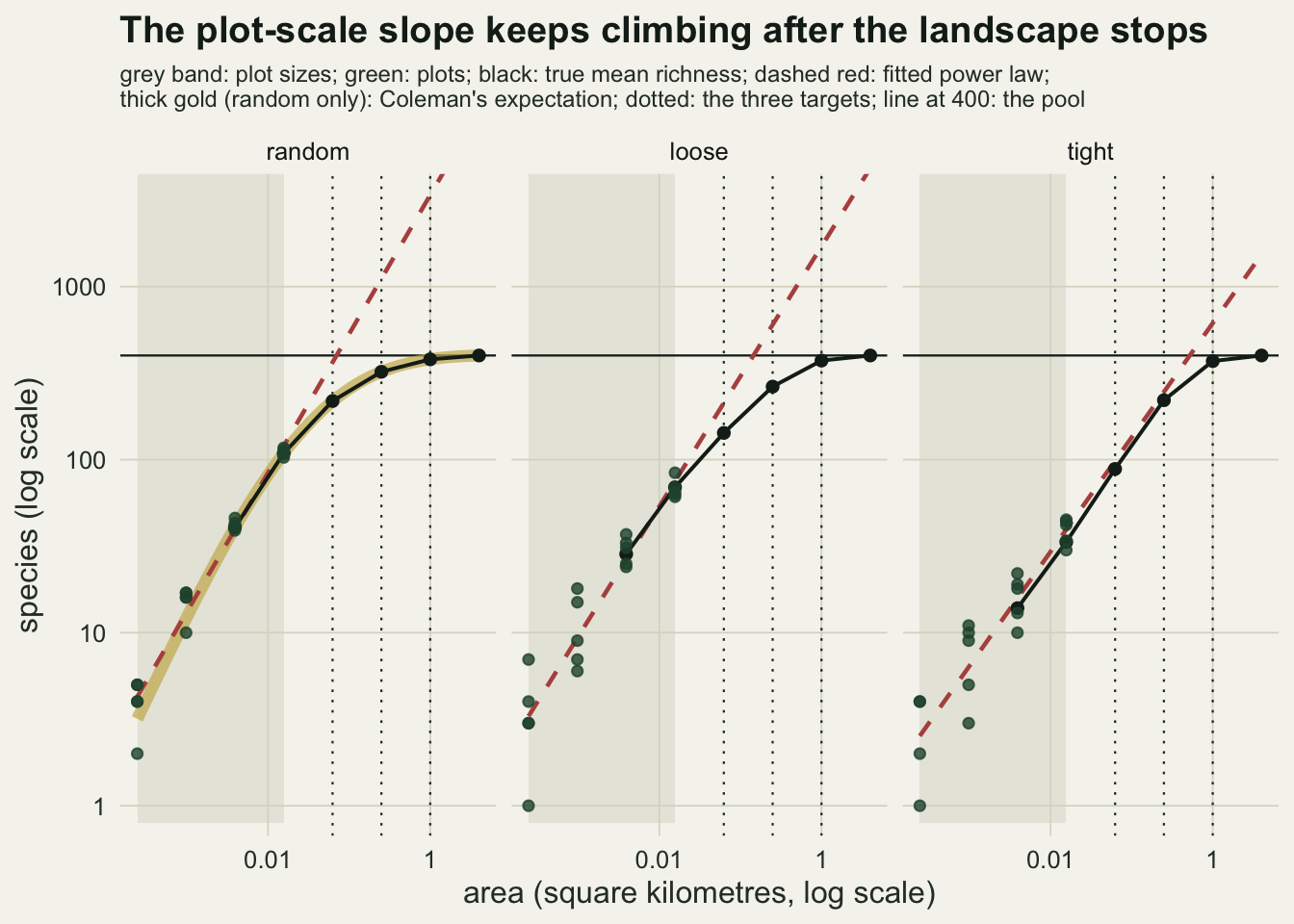
The power law wins the comparison and misses the target
Every landscape gets the same treatment: the twenty plots are fitted with a log-log power law and with the Gleason model (richness linear in log area), the two are compared by AIC with the Jacobian of the log transform added to the power law so that both likelihoods are on the richness scale, and both are run out to the three targets. The replication is 100 landscapes per cell, fixed before any cell was run, for three placements and two abundance distributions.
n_col  <- 320
f_grid <- c(0.05, 0.10, 0.25, 0.50, 0.75, 0.90)
m_grid <- c(2, 5, 10)

strip_loss <- function(w, z_across) {
  col_idx <- floor(w$x / side_dom * n_col)
  cnt <- matrix(tabulate(w$sp + col_idx * w$n_sp, w$n_sp * n_col), w$n_sp, n_col)
  two <- cbind(cnt, cnt)
  run <- matrix(cumsum(t(two)), nrow = w$n_sp, byrow = TRUE)
  run <- run - c(0, run[-w$n_sp, 2 * n_col])   # restart the running sum in each row
  cum <- cbind(0, run)
  do.call(rbind, lapply(f_grid, function(f) {
    keep <- round((1 - f) * n_col)
    left <- cum[, seq_len(n_col) + keep, drop = FALSE] - cum[, seq_len(n_col), drop = FALSE]
    data.frame(f = f, gone = mean(colSums(left == 0)),
               closed = sum(f^w$n_ind),
               sar_pred = w$n_sp * (1 - (1 - f)^z_across),
               comm2 = mean(colSums(left < 2 & w$n_ind >= 2)),
               comm5 = mean(colSums(left < 5 & w$n_ind >= 5)),
               comm10 = mean(colSums(left < 10 & w$n_ind >= 10)))
  }))
}

one_world <- function(n_sp, meanlog, placement, do_loss = TRUE) {
  w  <- make_world(n_sp, meanlog, placement)
  wr <- window_rich(w)
  pl <- nested_plots(w)
  pl <- pl[pl$rich > 0, ]
  pw <- lm(log(rich) ~ log(area), pl)
  gl <- lm(rich ~ log(area), pl)
  aic_pow <- AIC(pw) + 2 * sum(log(pl$rich))   # Jacobian: both on the richness scale
  aic_gle <- AIC(gl)
  truth <- wr$rich[match(tgt_area, wr$area)]
  pint  <- exp(predict(pw, data.frame(area = tgt_area), interval = "prediction"))
  pgle  <- predict(gl, data.frame(area = tgt_area))
  # one series of four plots: nested from one corner, or each size from its own origin
  one_nest  <- pl[pl$series == 1, ]
  one_indep <- pl[pl$series == match(pl$area, fit_area) + 1, ]
  pred_one <- function(d) exp(predict(lm(log(rich) ~ log(area), d),
                                      data.frame(area = max(tgt_area))))
  z_local <- diff(log(wr$rich[4:6])) / diff(log(wr$area[4:6]))
  z_across <- unname(coef(lm(log(rich) ~ log(area), wr[wr$area >= area_dom / 256, ]))[2])
  ext <- data.frame(placement, meanlog, n_sp, mult = tgt_mult,
                    pool = n_sp, truth = truth,
                    z_fit = unname(coef(pw)[2]), z_top = z_local[1],
                    r_pow = pint[, 1] / truth, r_gle = pgle / truth,
                    over_pool = pint[, 1] > n_sp,
                    cover = pint[, 2] <= truth & truth <= pint[, 3],
                    pi_width = pint[, 3] / pint[, 2],
                    above = pint[, 2] > truth,
                    pow_wins = aic_pow < aic_gle,
                    r_nest1 = pred_one(one_nest) / truth[3],
                    r_indep1 = pred_one(one_indep) / truth[3],
                    row.names = NULL)
  loss <- NULL
  if (do_loss) loss <- data.frame(placement, meanlog, z_across = z_across,
                                  single = sum(w$n_ind == 1), below5 = sum(w$n_ind < 5),
                                  strip_loss(w, z_across))
  list(ext = ext, loss = loss)
}
n_world <- 100
cells <- expand.grid(placement = c("random", "loose", "tight"), meanlog = c(2.5, 4),
                     stringsAsFactors = FALSE)
set.seed(5501)
runs <- unlist(lapply(seq_len(nrow(cells)), function(i)
  lapply(seq_len(n_world), function(r) one_world(400, cells$meanlog[i], cells$placement[i]))),
  recursive = FALSE)
ext_all  <- do.call(rbind, lapply(runs, `[[`, "ext"))
loss_all <- do.call(rbind, lapply(runs, `[[`, "loss"))
q_lo <- function(v) unname(quantile(v, 0.1))
q_hi <- function(v) unname(quantile(v, 0.9))
ext_med <- aggregate(cbind(r_pow, r_gle, truth, z_fit, z_top, pi_width) ~ placement + meanlog + mult,
ext_all, median)
ext_lo <- aggregate(cbind(r_pow, r_gle) ~ placement + meanlog + mult, ext_all, q_lo)
ext_hi <- aggregate(cbind(r_pow, r_gle) ~ placement + meanlog + mult, ext_all, q_hi)
ext_rate <- aggregate(cbind(cover, above, over_pool, pow_wins) ~ placement + meanlog + mult,
ext_all, mean)
pick <- function(tab, column, pl, ml, mu = 64) tab[[column]][tab$placement == pl & tab$meanlog == ml & tab$mult == mu]
aic_min <- min(ext_rate$pow_wins); aic_max <- max(ext_rate$pow_wins)
aic_mean <- mean(ext_all$pow_wins[ext_all$mult == 4])
mc_se_rate <- sqrt(0.25 / n_world)
pool_share <- aggregate(truth ~ placement + meanlog + mult, ext_all, median)
pool_share$share <- pool_share$truth / 400
share_16_min <- min(pool_share$share[pool_share$mult == 16])
share_64_min <- min(pool_share$share[pool_share$mult == 64])
# share of the variance of log(predicted / true) explained by each design factor alone
log_ratio <- log(ext_all$r_pow)
var_share <- sapply(c(placement = "placement", mult = "mult", meanlog = "meanlog"), function(v) {
grp <- ave(log_ratio, ext_all[[v]])
sum((grp - mean(log_ratio))^2) / sum((log_ratio - mean(log_ratio))^2)
})AIC prefers the power law in 97 per cent of all 600 landscapes, and in no cell in fewer than 92 per cent. By the criterion the species-area post uses, the power law is the right model nearly every time.
Under random placement with the rare-heavy pool, the power law predicts 1.84 times the true richness at 4 times the largest plot, 4.11 times at 16 and 11.4 times at 64 (medians over landscapes). Loose clusters give 1.63, 2.63 and 5.44. Tight clusters give 0.94, 0.95 and 1.41. With the less rare-heavy pool the random arm gives 2.00, 4.41 and 10.8, and the tight arm 0.87, 0.82 and 1.14.
So the error is not a fixed overshoot. It grows with the extrapolation multiple in the random and loose landscapes, it is small at 4 and 16 times in the tight ones, and in tight clusters with the second pool the median prediction is too low at the two nearer targets and too high at the far one, although single tight landscapes err in either direction (the bars in the figure cross 1). On these landscapes the degree of aggregation sets the size of the error and, in the median, its direction. Part of the far overshoot belongs to the landscape rather than to the power law: every species in the pool is present somewhere in the 4 square kilometres, and the median true richness at 16 times the largest plot is already at least 55 per cent of the 400 species in every cell, at 64 times at least 92 per cent. The 16 and 64 times ratios are therefore largely numbers about a line running past a saturated pool, and they would be smaller where larger areas add new habitats and new species.
The Gleason model is no rescue. Its median ratio at 64 times is 0.52, 0.35 and 0.16 for random, loose and tight with the first pool, and 1.06, 0.63 and 0.23 with the second. It errs low where the power law errs high, and its one near-correct cell is the random landscape with few rare species, which is one of the two cells where the power law is worst.
rat_df <- rbind(
  data.frame(model = "power law", ext_med[, c("placement", "meanlog", "mult")],
             med = ext_med$r_pow, lo = ext_lo$r_pow, hi = ext_hi$r_pow),
  data.frame(model = "Gleason", ext_med[, c("placement", "meanlog", "mult")],
             med = ext_med$r_gle, lo = ext_lo$r_gle, hi = ext_hi$r_gle))
rat_df$placement <- factor(rat_df$placement, levels = lev)
rat_df$pool <- factor(ifelse(rat_df$meanlog == 2.5, "log mean 2.5: many rare species",
                             "log mean 4: few rare species"))
rat_df$model <- factor(rat_df$model, levels = c("power law", "Gleason"))
dodge_x <- c(random = 0.88, loose = 1, tight = 1.14)
rat_df$x_pos <- rat_df$mult * dodge_x[as.character(rat_df$placement)]

ggplot(rat_df, aes(x_pos, med, colour = placement, shape = model)) +
  geom_hline(yintercept = 1, linetype = "dashed", colour = te_body, linewidth = 0.6) +
  geom_errorbar(aes(ymin = lo, ymax = hi), width = 0, linewidth = 0.6) +
  geom_line(aes(group = interaction(placement, model), linetype = model), linewidth = 0.7) +
  geom_point(size = 2.4) +
  facet_wrap(~ pool) +
  scale_colour_manual(values = place_col, name = NULL) +
  scale_linetype_manual(values = c("solid", "dotted"), name = NULL) +
  scale_shape_manual(values = c(16, 1), name = NULL) +
  scale_x_log10(breaks = c(4, 16, 64)) +
  scale_y_log10(breaks = c(0.1, 0.3, 1, 3, 10, 30)) +
  labs(x = "target area as a multiple of the largest plot",
       y = "predicted / true richness (log scale)",
       title = "Aggregation and the pool set the size of the error",
       subtitle = "dashed line: a correct prediction") +
  theme_datasheet() +
  theme(legend.position = "bottom")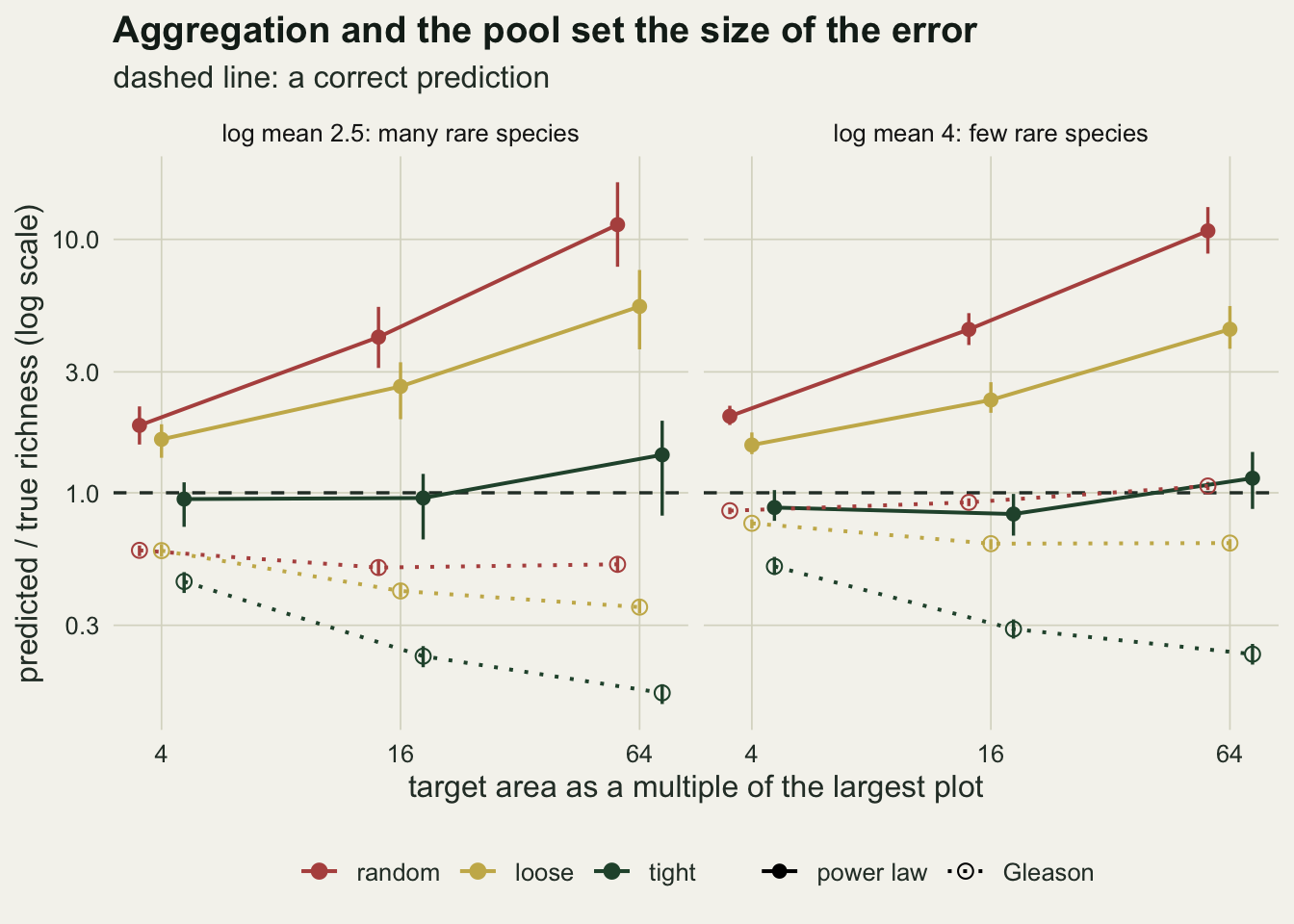
Why the plot-scale slope is the wrong slope
z_fit_rand <- pick(ext_med, "z_fit", "random", 2.5)
z_fit_tight <- pick(ext_med, "z_fit", "tight", 2.5)
z_top_rand <- pick(ext_med, "z_top", "random", 2.5)
z_top_tight <- pick(ext_med, "z_top", "tight", 2.5)
share_4_rand <- pick(pool_share, "share", "random", 2.5, 4)
over_pool_16 <- min(ext_rate$over_pool[ext_rate$mult == 16 & ext_rate$placement != "tight"])
over_pool_16_max <- max(ext_rate$over_pool[ext_rate$mult == 16 & ext_rate$placement != "tight"])
over_pool_tight <- pick(ext_rate, "over_pool", "tight", 2.5, 64)
The fitted exponent is steep. Its median is 0.86 in the random landscapes and 0.66 in the tight ones with the first pool, far above the textbook range of 0.15 to 0.35 quoted in the species-area post. That is not a fitting error. At 244 square metres a plot holds a handful of individuals, and every extra individual has a good chance of being a new species, so richness climbs almost in proportion to area: this is the sampling phase at the bottom of Preston’s curve. The slope of the true curve between the two largest targets, 25 hectares and one square kilometre, is 0.117 in the random landscapes and 0.377 in the tight ones. A straight line on log-log axes carries the first slope into the range where the second one holds.
The flat top is also where the question changes. The median true richness of the one square kilometre target is at least 92 per cent of the 400 species in the whole landscape in every cell, so predicting it is predicting the size of the species pool, the job of the asymptotic richness estimators, not the job of a curve through plot counts. Even 6.25 hectares already holds 55 per cent of the pool in the random landscapes with many rare species. The power law has no ceiling in it: at 16 times the largest plot its prediction exceeds the entire pool of 400 species in every random and loose landscape, and at 64 times it does so in 80 per cent of the tight landscapes with many rare species, where the median ratio still looked tolerable.
Clustering helps the power law for a reason that has nothing to do with the power law being the right shape. Tight clusters lower richness in small plots, since a plot either lands in a species’ cluster or it does not, and they delay the approach to the pool, so the true curve stays steep for longer and the plot-scale slope happens to be closer to the slope over the extrapolated range. The degree of clustering in a real landscape is not known from twenty plots, which is the practical content of the result.
An interval from the plots is honest only by accident
The obvious defence is the prediction interval: the fitted line is uncertain, and a 95 per cent interval on the log scale should say how far to trust it. Because the error is one-sided in most cells, the only informative check is two-sided coverage, together with the direction of the misses.
cov_rand_4  <- pick(ext_rate, "cover", "random", 2.5, 4)
cov_loose_4 <- pick(ext_rate, "cover", "loose", 2.5, 4)
cov_loose_4b <- pick(ext_rate, "cover", "loose", 4, 4)
cov_rand_4b <- pick(ext_rate, "cover", "random", 4, 4)
cov_loose_16 <- pick(ext_rate, "cover", "loose", 2.5, 16)
far_rows <- ext_all$mult == 64 & ext_all$placement != "tight"
n_far <- sum(far_rows)
n_far_cover <- sum(ext_all$cover[far_rows])
n_far_above <- sum(ext_all$above[far_rows])
bias_tight_64 <- pick(ext_med, "r_pow", "tight", 2.5, 64)
bias_rand_64 <- pick(ext_med, "r_pow", "random", 2.5, 64)
near_rows <- ext_rate$mult == 4 & ext_rate$placement != "tight"
near_cov_min <- min(ext_rate$cover[near_rows]); near_cov_max <- max(ext_rate$cover[near_rows])
near_bias_min <- min(ext_med$r_pow[ext_med$mult == 4 & ext_med$placement != "tight"])
near_bias_max <- max(ext_med$r_pow[ext_med$mult == 4 & ext_med$placement != "tight"])
cov_tight_min <- min(ext_rate$cover[ext_rate$placement == "tight"])
width_tight_64 <- pick(ext_med, "pi_width", "tight", 2.5, 64)
width_rand_64 <- pick(ext_med, "pi_width", "random", 2.5, 64)
With the first pool, the interval covers the true richness at 4 times the largest plot in 80 per cent of random landscapes and 99 per cent of loose ones; with the second pool those fall to 1 and 69 per cent. At 16 times the loose landscapes manage 31 per cent, and at 64 times 0 of the 400 random and loose landscapes are covered, with the whole interval above the truth in 400 of them. The Monte Carlo standard error of any of these rates is at most 0.050.
The tight landscapes look like the success story: coverage is at least 98 per cent at every multiple and for both pools. The interval did not earn it. Tight clusters make plot richness erratic between series, so the median interval at 64 times spans a factor of 8.8 from its lower to its upper end, against 5.9 in the random landscapes. That is wider, but not different in kind: the random interval misses a median bias of 11.4 times, and the tight interval covers a median bias of 1.41 times, while its central prediction exceeds the whole species pool in 80 per cent of those landscapes. Coverage follows the size of the bias, and nothing in the plot data tells the analyst which kind of landscape they are in. No interval from a plot-scale fit is trustworthy beyond the fitted range, and the recommendation that survives is a limit on the multiple rather than a better interval.
nest_med  <- aggregate(cbind(r_nest1, r_indep1) ~ placement + meanlog, ext_all[ext_all$mult == 64, ], median)
nest_lo   <- aggregate(cbind(r_nest1, r_indep1) ~ placement + meanlog, ext_all[ext_all$mult == 64, ], q_lo)
nest_hi   <- aggregate(cbind(r_nest1, r_indep1) ~ placement + meanlog, ext_all[ext_all$mult == 64, ], q_hi)
nest_gap  <- max(abs(log(nest_med$r_nest1 / nest_med$r_indep1)))
pk2 <- function(tab, column, pl, ml) tab[[column]][tab$placement == pl & tab$meanlog == ml]

set.seed(7707)
pool_sizes <- c(200, 800)
n_world_pool <- 30
pool_runs <- do.call(rbind, lapply(pool_sizes, function(s_pool)
  do.call(rbind, lapply(c("random", "loose", "tight"), function(pl)
    do.call(rbind, lapply(seq_len(n_world_pool), function(r)
      one_world(s_pool, 2.5, pl, do_loss = FALSE)$ext))))))
pool_med <- aggregate(r_pow ~ placement + n_sp + mult, pool_runs, median)
pool_pick <- function(pl, s_pool, mu = 64) pool_med$r_pow[pool_med$placement == pl & pool_med$n_sp == s_pool & pool_med$mult == mu]
Two design choices could be suspected of producing the result. The first is the nested series. A field design with each plot size at its own random origin gives the same expected richness at every size, because expected richness depends only on area, so it should move the variance and not the sign. Fitting a single series of four plots, either nested from one corner or with each size taken from a different series, gives median ratios at 64 times of 9.7 and 12.0 in the random landscapes and 1.28 and 1.37 in the tight ones with the first pool; the largest gap between the two designs across all six cells is a factor of 1.23. The 10 to 90 per cent range for a single tight series at 64 times runs from 0.50 to 3.14 with independent origins, so in a single tight landscape the error can take either sign whichever design is used.
The second is the pool of 400 species. Rerunning the extrapolation with 30 landscapes each for pools of 200 and 800 species, with the first abundance distribution, gives median ratios at 64 times of 10.5 and 10.9 for random placement, 4.3 and 5.2 for loose clusters, and 0.94 and 1.49 for tight clusters. The random and loose ratios change far less than the gap between placements; the tight ratio moves from one side of a correct prediction to the other on only 30 landscapes, which is the same instability the single-series range shows.
cov_df <- ext_rate
cov_df$placement <- factor(cov_df$placement, levels = lev)
cov_df$pool <- factor(ifelse(cov_df$meanlog == 2.5, "log mean 2.5: many rare species",
                             "log mean 4: few rare species"))
ggplot(cov_df, aes(mult, cover, colour = placement)) +
  geom_hline(yintercept = 0.95, linetype = "dashed", colour = te_body, linewidth = 0.6) +
  geom_line(linewidth = 0.9) +
  geom_point(size = 2.6) +
  facet_wrap(~ pool) +
  scale_colour_manual(values = place_col, name = NULL) +
  scale_x_log10(breaks = c(4, 16, 64)) +
  scale_y_continuous(limits = c(0, 1)) +
  labs(x = "target area as a multiple of the largest plot",
       y = "share of landscapes covered",
       title = "Coverage follows the bias, not the interval",
       subtitle = "dashed line: the nominal 95 per cent") +
  theme_datasheet() +
  theme(legend.position = "bottom")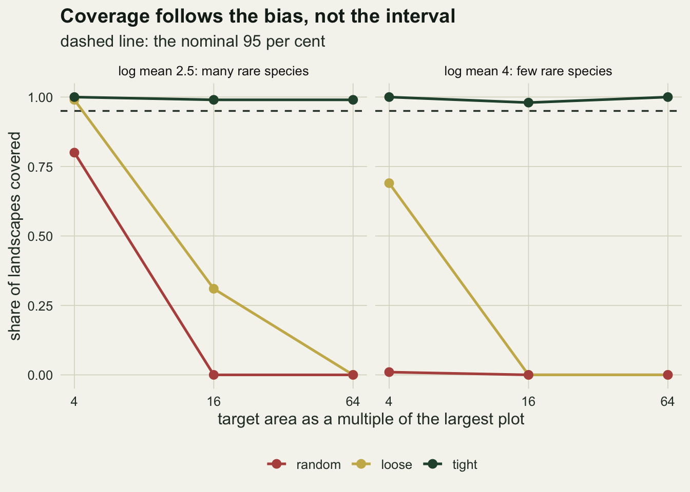
Running the curve backwards
The same fitted curve is used in the other direction to estimate extinctions from habitat loss: if a fraction f of the area is destroyed, a power law with exponent z predicts that S times one minus (1 - f) to the power z species are lost. He and Hubbell argued in 2011 that this always overestimates the species lost at the moment of destruction, because a species is lost only when every one of its individuals was in the destroyed part, and that is a different curve, the endemics-area relationship. Pereira, Borda-de-Agua and Martins replied in 2012 that the comparison depends on geometry and scale, and Kitzes and Harte showed in 2014 that extinction forecasts shift a great deal with the minimum abundance a species needs to count as surviving.
Some of this is plain arithmetic. For any placement of individuals, the species gone when part of a landscape is destroyed are the S species minus the richness of what is left, so the true species-area curve read backwards on the same geometry gives exactly the endemics-area number. Under random placement both also have a closed form: a species with N individuals has all of them in the destroyed fraction with probability f to the power N, so the expected loss is the sum of f to the N over species, which is S minus Coleman’s expected richness of the remaining area. What overshoots is a power law, because its z is a single slope and the real curve flattens at the top.
Loss here is a contiguous strip of the landscape, averaged over all 320 strip positions on a grid of 6.25 metre columns. The exponent is fitted in the way a regional study would fit it, across window sizes from a 256th of the landscape up to the whole of it. Committed loss counts species that start with at least m individuals and are left with fewer than m, for m of 2, 5 and 10; it is a threshold proxy for species doomed to go later, not a demographic model.
loss_mean <- aggregate(cbind(z_across, single, below5, gone, closed, sar_pred, comm2, comm5, comm10) ~
                         placement + meanlog + f, loss_all, mean)
loss_mean$ratio_gone <- loss_mean$sar_pred / loss_mean$gone
pick_f <- function(column, pl, ml, fr) loss_mean[[column]][loss_mean$placement == pl & loss_mean$meanlog == ml & abs(loss_mean$f - fr) < 1e-9]

rand_rows <- loss_all[loss_all$placement == "random", ]
closed_gap <- aggregate(cbind(gone, closed) ~ meanlog + f, rand_rows, mean)
closed_se  <- aggregate(gone ~ meanlog + f, rand_rows, function(v) sd(v) / sqrt(length(v)))
closed_z   <- max(abs(closed_gap$gone - closed_gap$closed) / pmax(closed_se$gone, 1e-9))
single_f10 <- pick_f("single", "random", 2.5, 0.1) * 0.1
# Monte Carlo SE of the mean immediate loss, relative to the mean, at 10 per cent loss
gone_rse <- aggregate(gone ~ placement + meanlog + f, loss_all, function(v) sd(v) / sqrt(length(v)) / mean(v))
rse_f10 <- function(ml) range(gone_rse$gone[gone_rse$meanlog == ml & abs(gone_rse$f - 0.1) < 1e-9])
single_4 <- range(loss_mean$single[loss_mean$meanlog == 4 & abs(loss_mean$f - 0.1) < 1e-9])
gone4 <- range(loss_mean$gone[loss_mean$meanlog == 4 & abs(loss_mean$f - 0.1) < 1e-9])
sig2 <- function(v) sprintf("%.0f", signif(v, 2))
# how far the ratio moves with the abundance distribution (fixed f) and with f (fixed cell)
sad_fac <- function(fr) range(sapply(lev, function(pl) pick_f("ratio_gone", pl, 4, fr) / pick_f("ratio_gone", pl, 2.5, fr)))
f_fac <- range(sapply(lev, function(pl) sapply(c(2.5, 4), function(ml)
  pick_f("ratio_gone", pl, ml, 0.05) / pick_f("ratio_gone", pl, ml, 0.9))))
The closed form holds. In the random landscapes the mean simulated loss and the mean of the sum of f to the N differ by at most 0.9 Monte Carlo standard errors over all twelve combinations of loss fraction and abundance distribution; at half the landscape lost, with the first pool, they are 4.26 and 4.15 species.
The power law’s predictions are far larger. With the first pool and 10 per cent of the landscape destroyed, it predicts 9.4 species lost in the random landscapes, where 0.34 are actually lost: a ratio of 28. The loose and tight landscapes give ratios of 37 and 48. With the second pool, which has hardly any rare species, the same ratios are about 190, 400 and 770. At 90 per cent loss they shrink to 3.4, 2.9 and 2.3 with the first pool and 9.0, 5.9 and 3.3 with the second. The second-pool ratios at 10 per cent loss are fragile: their denominator is an immediate loss of about 0.021 species per landscape, which rests on 0.08 to 0.15 singleton species per landscape on average, or 8 to 15 singleton species in all 100 landscapes of a cell. The Monte Carlo standard error of that mean loss is 18 to 22 per cent of it, against 5 to 6 per cent with the first pool, and the immediate loss is nearly the same in all three placements (0.0206 to 0.0209 species), so the ordering of those three ratios comes from the power law’s prediction, not from the loss. How many singletons there are is itself a design choice here: every species gets one individual plus a Poisson draw on a 4 square kilometre landscape.
Two things set the size of the ratio. For small f the sum of f to the N is dominated by species with one individual, so the true immediate loss is close to f times the number of singletons: the first pool averages 2.89 singletons among 400 species, so f times that at 10 per cent is 0.29, against the 0.34 lost. A pool with fewer singletons has a much smaller denominator: in the random landscapes at 10 per cent loss the ratio rises from 28 to about 190 even though the power law’s own prediction falls from 9.4 to 4.0 species; at 5 per cent loss the second pool multiplies the ratio by 7.9 to 18.2 across the three placements. The loss fraction matters as much or more: between 5 and 90 per cent loss the ratio falls by a factor of 8.5 to 296 across the six cells, and at 90 per cent the second pool multiplies it by only 1.4 to 2.6. One ratio quoted from one simulated community at one loss fraction says very little.
bw_df <- loss_mean
bw_df$placement <- factor(bw_df$placement, levels = lev)
bw_df$pool <- factor(ifelse(bw_df$meanlog == 2.5, "log mean 2.5: many rare species",
                            "log mean 4: few rare species"))
ggplot(bw_df, aes(f, ratio_gone, colour = placement)) +
  geom_hline(yintercept = 1, linetype = "dashed", colour = te_body, linewidth = 0.6) +
  geom_line(linewidth = 0.9) +
  geom_point(size = 2.4) +
  facet_wrap(~ pool) +
  scale_colour_manual(values = place_col, name = NULL) +
  scale_y_log10(breaks = c(1, 3, 10, 30, 100, 300, 1000)) +
  labs(x = "fraction of the landscape destroyed (one contiguous strip)",
       y = "predicted / actual species lost (log scale)",
       title = "The backward overshoot is largest when little is lost",
       subtitle = "means over 100 landscapes per cell; dashed line: a correct prediction") +
  theme_datasheet() +
  theme(legend.position = "bottom")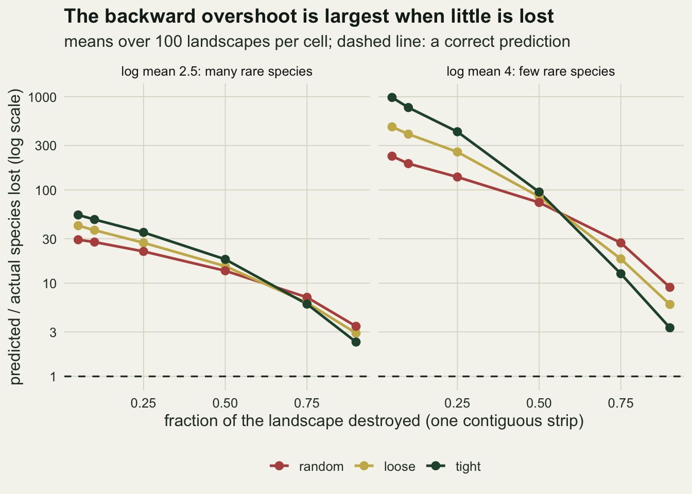
If the species-area number is read as a count of species committed to extinction rather than lost at once, the comparison depends on the threshold.
comm_tab <- loss_mean[loss_mean$f %in% c(0.1, 0.5) , c("placement", "meanlog", "f", "sar_pred", "gone", "comm2", "comm5", "comm10")]
comm_tab <- comm_tab[order(comm_tab$meanlog, comm_tab$f, match(comm_tab$placement, lev)), ]
print(format(comm_tab, digits = 3), row.names = FALSE)
placement meanlog f sar_pred gone comm2 comm5 comm10
random 2.5 0.1 9.39 0.3401 1.0997 3.770 6.64
loose 2.5 0.1 12.95 0.3498 1.1083 3.724 7.17
tight 2.5 0.1 18.95 0.3930 1.2045 3.915 7.02
random 2.5 0.5 57.89 4.2616 11.2701 31.414 52.12
loose 2.5 0.5 77.87 5.1191 12.9336 35.476 57.76
tight 2.5 0.5 109.32 6.0659 14.5408 36.515 58.61
random 4.0 0.1 3.97 0.0207 0.0766 0.469 1.30
loose 4.0 0.1 8.32 0.0209 0.0966 0.495 1.42
tight 4.0 0.1 15.81 0.0206 0.1053 0.619 1.52
random 4.0 0.5 25.39 0.3459 1.2223 5.356 13.88
loose 4.0 0.5 51.64 0.6094 1.7506 6.889 16.94
tight 4.0 0.5 93.19 0.9805 2.2783 7.922 17.72below5_a <- pick_f("below5", "random", 2.5, 0.1)
below5_b <- pick_f("below5", "random", 4, 0.1)
small_f <- loss_mean[abs(loss_mean$f - 0.1) < 1e-9, ]
c10_a <- range(small_f$sar_pred[small_f$meanlog == 2.5] / small_f$comm10[small_f$meanlog == 2.5])
c10_b <- range(small_f$sar_pred[small_f$meanlog == 4] / small_f$comm10[small_f$meanlog == 4])With the first pool and half the random landscape destroyed, the power law predicts 57.9 species lost, and the committed counts are 11.3, 31.4 and 52.1 at thresholds of 2, 5 and 10 individuals. Only the highest threshold comes near the power law’s figure, and only at a large loss. At 10 per cent loss the power law exceeds even the count below 10 individuals by a factor of 1.4 to 2.7 with the first pool and 3.0 to 10.4 with the second. At half the random landscape lost with the first pool, the power law is 5.1 times the committed count at a threshold of 2 and 1.11 times the count at 10. How large an overestimate the species-area number looks is set by the threshold chosen, which is the sensitivity Kitzes and Harte describe. The threshold also meets the pool before any loss happens, since on average 19.4 of the 400 species in the first pool and 1.9 in the second start with fewer than 5 individuals and are left out of the committed count altogether.
What to report
Report the areas of the plots and the areas of the targets as a multiple of the largest plot, in the same sentence as the predicted richness. On these landscapes the placement of individuals alone accounts for 58 per cent of the variance of the log ratio of predicted to true richness and the multiple alone for 28 per cent; the placement cannot be read from twenty plots, but the multiple can be reported, and a reader cannot reconstruct it from a fitted exponent.
Give the fitted exponent with the range of areas it came from. An exponent of 0.52 to 0.86 (the range of the cell medians here) from plots of a few hundred square metres is a statement about sampling individuals, and quoting it next to published regional exponents of 0.15 to 0.35 invites a comparison that has no meaning.
Do not report a prediction interval from a plot-scale fit as the uncertainty of a regional richness. Where the interval covered here, it did so because the bias happened to be small in that kind of landscape, not because the interval measured the bias. If a number for a larger area is needed, state it as a lower bound from the largest plots plus a pool estimate from abundance or incidence data, and say that the curve was not used past the fitted range; even at 4 times the largest plot the median ratio in the random and loose landscapes was 1.54 to 2.00 and coverage ran from 1 to 99 per cent, so no multiple past the fitted range was safe on these landscapes.
For habitat loss, say which quantity the number is: species gone at once, species below a named threshold, or a curve evaluated past its data. Give the fraction of area lost and the abundance distribution, or at least the number of species known from one or two individuals: at small losses the singletons set the ratio between the power law and the immediate loss, and the ratio falls steeply as the loss grows.
Honest limits
The landscapes are stationary and homogeneous: species differ in abundance and aggregation, but no species tracks an environmental gradient and there is no turnover between habitats. Real regional richness grows partly because larger areas include new habitats, which keeps the top of the curve steeper than here, and a plot-scale slope may then overshoot less. The result to carry is that the error depends on structure the plots cannot reveal, not the particular ratios.
The truth used for the targets is the mean richness over every square of that size, while the prediction interval is for one new square. For the random landscapes that difference is small next to the bias, but for tight clusters the richness of one particular one square kilometre compartment varies more, and the coverage figures should be read as coverage of the landscape mean.
Clustering is one Thomas-type process with the same mean number of cluster centres for every species. Real species differ in range size, and the rare species are often the most restricted, which would make the pool approach slower. The two abundance distributions bracket a rare-heavy and a rare-poor pool without claiming that either is typical.
Only the two classical curves were fitted. Saturating models, the random placement formula fitted to plot abundances, and the occupancy-at-several-grains upscaling methods compared by Kunin and colleagues use more information than a count per plot, and Kunin and colleagues compared many such methods on real data; none was tested here, so this post cannot say whether they would beat the two curves on these landscapes.
The backward section uses one loss geometry, a contiguous strip. Loss in scattered cells removes the aggregated species less completely and would probably move the clustered arms towards the random one; that was not run. The committed counts are thresholds on individuals left anywhere in the remaining landscape, with no demography, no connectivity and no time to extinction.
References
Preston FW 1960 Ecology 41(4):611-627 (10.2307/1931793)
Coleman BD 1981 Mathematical Biosciences 54(3-4):191-215 (10.1016/0025-5564(81)90086-9)
Plotkin JB, Potts MD, Yu DW, et al. 2000 Proceedings of the National Academy of Sciences 97(20):10850-10854 (10.1073/pnas.97.20.10850)
Kunin WE, Harte J, He F, et al. 2018 Ecological Monographs 88(2):170-187 (10.1002/ecm.1284)
He F, Hubbell SP 2011 Nature 473(7347):368-371 (10.1038/nature09985)
Pereira HM, Borda-de-Agua L, Martins IS 2012 Nature 482(7386):E3-E4 (10.1038/nature10857)
Kitzes J, Harte J 2014 Methods in Ecology and Evolution 5(1):1-8 (10.1111/2041-210x.12130)