Checking a metapopulation model

Three diagnostics for a spatial metapopulation model in R: the equilibrium assumption, a weakly identified dispersal kernel, and stochastic extinction risk.

Corrected 8 October 2026: the profile caption called the dispersal kernel almost unidentified, where its likelihood interval is bounded on both sides, and now calls it weakly identified; the stochastic check now says that where its risk switches on also depends on a horizon that is very long against the lifetime of a single patch, and the code comment no longer implies that the time step is short against the patch extinction rates.

Corrected 1 October 2026: the stochastic check used a time step so long that nearly every patch died within one step, so almost every extinction it counted happened in the first step and the risk came out as a smooth ramp; with a short step the risk is near zero at the lowest ratio and certain from a ratio of a half. The transient fit had stopped on a flat ridge of the likelihood and now keeps the best of several starts, which puts its area exponent at the edge of its range.

The three previous tutorials in this set are convenient to the point of being seductive. The incidence function model fits from a single snapshot; the metapopulation capacity boils a whole landscape down to one eigenvalue; the persistence rule is a clean inequality. Each convenience rests on an assumption that a snapshot cannot check on its own, and when the assumption fails the model does not complain: it returns a confident, wrong answer. This tutorial builds three diagnostics in base R for exactly those failure modes. It reuses the clustered landscape and the fitting machinery from the incidence function post, so the checks apply directly to what came before.

Efun <- function(A, mu, x) pmin(1, mu / A^x)
conn <- function(o, D, A, alpha) {
  M <- exp(-alpha * D) * outer(rep(1, length(A)), A)
  diag(M) <- 0
  as.numeric(M %*% o)
}
Cfun <- function(S, y) S^2 / (S^2 + y^2)

set.seed(2024)
K <- 6; per <- 26
centres <- cbind(runif(K, 3, 25), runif(K, 3, 25))
clus <- do.call(rbind, lapply(1:K, function(k)
  cbind(rnorm(per, centres[k, 1], 1.3), rnorm(per, centres[k, 2], 1.3))))
iso <- cbind(runif(44, 1, 27), runif(44, 1, 27))
patch <- rbind(clus, iso)
n <- nrow(patch)
A <- rlnorm(n, meanlog = 0, sdlog = 0.9)
D <- as.matrix(dist(patch))
mu_t <- 0.8; x_t <- 1.0; y_t <- 2.5; alpha_t <- 0.6
Etrue <- Efun(A, mu_t, x_t)

fitIFM <- function(o, af = 0.6) {
  S <- conn(o, D, A, af)
  nll <- function(p) {
    mu <- exp(p[1]); x <- exp(p[2]); y <- exp(p[3])
    C <- Cfun(S, y); E <- Efun(A, mu, x)
    J <- pmin(pmax(C / (C + E), 1e-9), 1 - 1e-9)
    -sum(dbinom(o, 1, J, log = TRUE))
  }
  # several starts, one with mu below one: where mu / A^x exceeds one for every
  # patch, E is capped at one and the likelihood is flat in x
  best <- NULL
  for (s in list(log(c(0.5, 1, 2)), log(c(1, 0.5, 1)), log(c(0.3, 1.5, 4)),
                 log(c(2, 1, 0.5)), log(c(0.7, 0.1, 4)))) {
    f <- optim(s, nll, method = "Nelder-Mead",
               control = list(maxit = 4000, reltol = 1e-12))
    f <- optim(f$par, nll, method = "BFGS")
    if (is.null(best) || f$value < best$value) best <- f
  }
  list(par = exp(best$par), ll = -best$value)
}
n

[1] 200

Check one: is the snapshot at equilibrium?

The incidence function model reads the balance of colonisation and extinction off the spatial pattern, on the assumption that the pattern is stationary. A recovering or collapsing network breaks that. To see the damage, fit two snapshots of the same landscape: one at stochastic equilibrium, and one taken while the network is still climbing back from a crash.

The equilibrium snapshot is the one from the incidence function tutorial, run to stationarity. The transient snapshot starts from five per cent occupied and runs only six gentle steps, so the network is a long way from settled. The gentle step (each rate scaled by a small factor) leaves the equilibrium unchanged but slows the approach, making the transient unambiguous.

o <- as.integer(runif(n) < 0.5)
set.seed(303)
for (t in 1:2000) {
  S <- conn(o, D, A, alpha_t); C <- Cfun(S, y_t)
  new <- o; emp <- o == 0L; occ <- o == 1L
  new[emp] <- as.integer(runif(sum(emp)) < C[emp])
  new[occ] <- as.integer(runif(sum(occ)) >= Etrue[occ])
  o <- new
}
o_eq <- o

tau <- 0.25
stepT <- function(o) {
  S <- conn(o, D, A, alpha_t); C <- Cfun(S, y_t)
  new <- o; emp <- o == 0L; occ <- o == 1L
  new[emp] <- as.integer(runif(sum(emp)) < C[emp] * tau)
  new[occ] <- as.integer(runif(sum(occ)) >= Etrue[occ] * tau)
  new
}
set.seed(505)
o <- as.integer(runif(n) < 0.05)
for (t in 1:6) o <- stepT(o)
o_tr <- o
c(equilibrium_occupied = sum(o_eq), transient_occupied = sum(o_tr))

equilibrium_occupied   transient_occupied 
                 117                   76 

The equilibrium snapshot has 117 occupied patches; the transient, still recovering, has 76. Now fit the incidence function model to each and compare with the truth (mu = 0.8, x = 1.0, y = 2.5).

fe <- fitIFM(o_eq); ft <- fitIFM(o_tr)
rbind(equilibrium = round(fe$par, 3),
      transient   = round(ft$par, 3))

             [,1]  [,2]  [,3]
equilibrium 0.441 0.841 3.620
transient   0.723 0.000 3.827

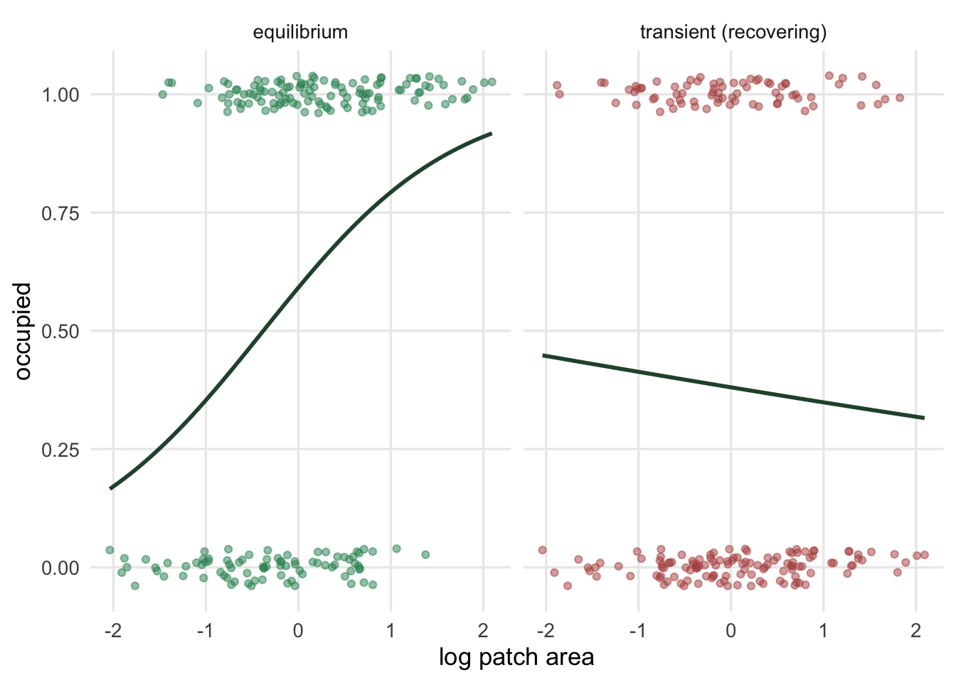
Fitted to the equilibrium snapshot, the area exponent x comes out at 0.841, against the true 1.0. The transient fit gives an area exponent x of 0, at the edge of what the model allows. Where that exponent comes out near zero it says extinction barely depends on area, and a conservation planner who read it that way would conclude, wrongly, that patch size hardly matters. Correlate occupancy with area and with connectivity in each snapshot.

S_eq <- conn(o_eq, D, A, alpha_t); S_tr <- conn(o_tr, D, A, alpha_t)
rbind(equilibrium = c(area = cor(o_eq, log(A)), connectivity = cor(o_eq, log(S_eq + 1e-6))),
      transient   = c(area = cor(o_tr, log(A)), connectivity = cor(o_tr, log(S_tr + 1e-6)))) |>
  round(3)

              area connectivity
equilibrium  0.356        0.298
transient   -0.056        0.376

At equilibrium, occupancy tracks area (correlation 0.36): large patches persist, small ones wink out, which is the extinction-area signal the model is built to read. At the transient, the area correlation is -0.056 while the connectivity correlation is 0.376. When recovery is driven by connectivity, the well-connected patches near the surviving core refill first, regardless of their size, and the snapshot carries little area signal for the model to find. The tell is simple: a near-zero area exponent from a system you have reason to think is disturbed should be read as a warning about equilibrium, not as biology.

Figure 1: Occupancy against patch area at equilibrium and during recovery from a crash. The trend line rises with area at equilibrium (extinction hits small patches) and is close to flat during recovery.

Check two: can the snapshot see the dispersal kernel?

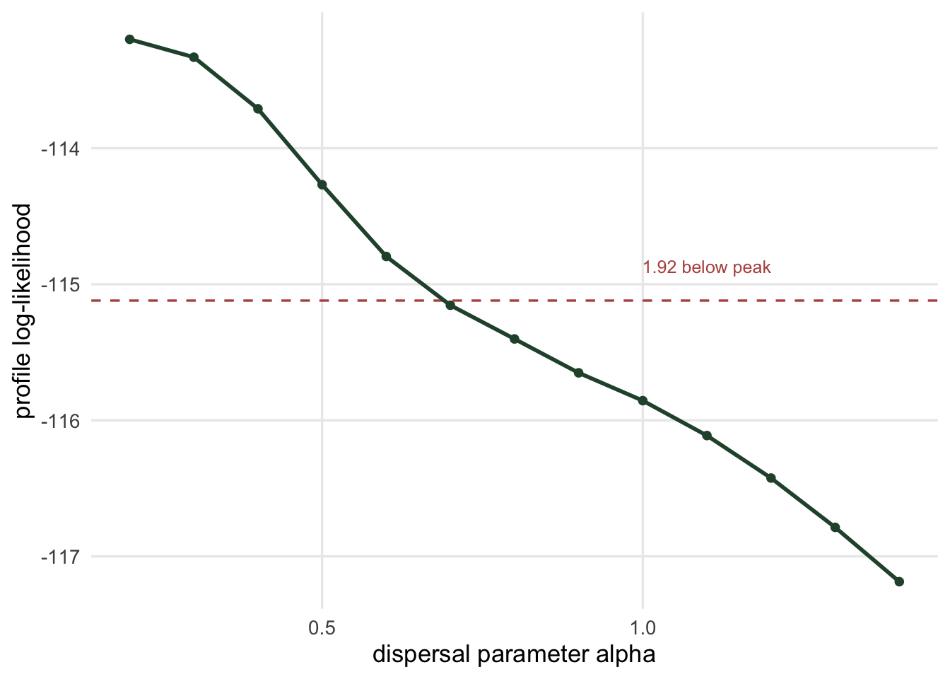
The incidence function tutorial fixed alpha by hand and promised an explanation. Here it is: a single snapshot barely constrains the dispersal parameter, yet the metapopulation capacity of the previous tutorial depends on it heavily. Profile the likelihood of the equilibrium snapshot over a range of alpha, re-fitting the other three parameters at each value.

proflik <- function(al) {
  Sa <- conn(o_eq, D, A, al)
  nl <- function(p) {
    mu <- exp(p[1]); x <- exp(p[2]); y <- exp(p[3])
    Cc <- Cfun(Sa, y); Ee <- Efun(A, mu, x)
    Jj <- pmin(pmax(Cc / (Cc + Ee), 1e-9), 1 - 1e-9)
    -sum(dbinom(o_eq, 1, Jj, log = TRUE))
  }
  starts <- list(log(c(0.5, 1, 2)), log(c(1, 0.5, 1)),
                 log(c(0.3, 1.5, 4)), log(c(2, 1, 0.5)))
  best <- Inf
  for (s in starts) {
    r <- optim(s, nl, method = "Nelder-Mead", control = list(maxit = 3000, reltol = 1e-11))
    r <- optim(r$par, nl, method = "BFGS")
    if (r$value < best) best <- r$value
  }
  -best
}
alg <- seq(0.05, 1.4, by = 0.05)
pl <- sapply(alg, proflik)
inb <- range(alg[pl >= max(pl) - 1.92])
c(logLik_span = round(max(pl) - min(pl), 2), ci_low = inb[1], ci_high = inb[2])

logLik_span      ci_low     ci_high 
       4.23        0.10        0.65 

Over a twenty-eight-fold range of alpha, the whole profile log-likelihood moves by only 4.23 units. Everything from alpha = 0.1 to 0.65 sits within the usual 1.92-unit interval, so the snapshot cannot tell a short kernel from one 6.5 times as wide. The true value, 0.6, sits 1.6 units below a profile that peaks at alpha = 0.2.

Figure 2: Profile log-likelihood for the dispersal parameter from a single snapshot. The curve is shallow: values across a wide range fall within the dashed interval line, so the snapshot leaves the kernel only weakly identified.

That shallow profile matters because the metapopulation capacity is not flat in alpha at all. Feeding the two ends of the interval into the capacity calculation shows how much rides on a parameter the data cannot pin down.

Mmat <- function(al) { M <- exp(-al * D) * outer(A, A); diag(M) <- 0; M }
lamOf <- function(al) eigen(Mmat(al), symmetric = TRUE, only.values = TRUE)$values[1]
c(lambda_at_low = round(lamOf(inb[1]), 1),
  lambda_at_high = round(lamOf(inb[2]), 1),
  fold_range = round(lamOf(inb[1]) / lamOf(inb[2]), 1))

 lambda_at_low lambda_at_high     fold_range 
         329.9           80.0            4.1 

The capacity ranges from 330 down to 80 across the plausible alpha, a 4.1-fold spread. Every persistence verdict and every patch-value ranking from the capacity tutorial inherits that uncertainty. The honest way to report a capacity from a snapshot is as a range this wide, not a single number, unless alpha has been fixed from independent dispersal data.

Check three: is the threshold a promise?

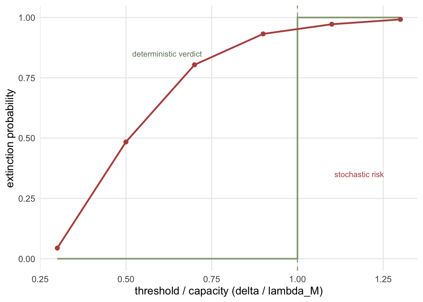
The capacity rule says persist when lambda_M exceeds the species threshold delta. That is a deterministic statement about an infinite system. A real metapopulation has finitely many patches and turns over by chance, so it can wink out even when the deterministic rule says it is safe. To measure the gap, simulate a spatially explicit stochastic model on the same landscape: each occupied patch goes extinct at a rate that falls with area, each empty patch is colonised at a rate that rises with connectivity, and we ask how often the whole network dies within a fixed horizon.

lamM <- lamOf(alpha_t)
K_t <- exp(-alpha_t * D) * outer(rep(1, n), A)   # the kernel conn() uses, built once
diag(K_t) <- 0
sim_srl <- function(cc, ee, steps, tau, seed) {
  set.seed(seed)
  o <- rep(1L, n)
  for (t in 1:steps) {
    S <- as.numeric(K_t %*% o)
    pc <- 1 - exp(-cc * S * tau); pe <- 1 - exp(-(ee / A) * tau)
    new <- o; emp <- o == 0L; occ <- o == 1L
    new[emp] <- as.integer(runif(sum(emp)) < pc[emp])
    new[occ] <- as.integer(runif(sum(occ)) >= pe[occ])
    o <- new
    if (sum(o) == 0) return(TRUE)
  }
  FALSE
}
# a step that is long against the extinction rates ee / A lets a fully occupied
# network empty in its first step; 0.01 is short enough to prevent that, though
# still coarse against ee / A for most patches, and 4000 steps of it cover the
# same 40 time units
cc <- 1; R <- 250; H <- 4000; tau_s <- 0.01
ratios <- c(0.3, 0.5, 0.7, 0.9, 1.1, 1.3)
pext <- sapply(ratios, function(rr) {
  ee <- rr * lamM * cc
  mean(sapply(1:R, function(k) sim_srl(cc, ee, H, tau_s, seed = 5000 + round(rr * 1000) + k)))
})
data.frame(delta_over_lambda = ratios, extinction_prob = round(pext, 3))

  delta_over_lambda extinction_prob
1               0.3            0.02
2               0.5            1.00
3               0.7            1.00
4               0.9            1.00
5               1.1            1.00
6               1.3            1.00

The deterministic rule is a step: safe below a ratio of one, doomed above it. The stochastic model has a step of its own, in a different place. At a ratio of 0.5 (that is, lambda_M twice the threshold, deep in the supposedly safe zone), the network dies out 100% of the time within the horizon, while at a ratio of 0.3 the extinction probability is 2%. The risk does not switch on at the threshold: on this landscape, and over a horizon that is very long against the lifetime of a single patch, it switches on well inside the safe side; a shorter horizon would move the switch towards the threshold, a longer one further in. The simulation has to resolve the turnover of patches to show this: with a time step that is long against the extinction rates, nearly every patch dies within one step, and a network that starts fully occupied can vanish in the first step, before any colonisation is possible.

Figure 3: Stochastic extinction probability against the ratio of species threshold to metapopulation capacity, with the deterministic verdict as a step. The deterministic rule flips from safe to doomed at a ratio of one; the simulated extinction risk is near zero at the lowest ratio and already certain at a ratio of a half, well on the safe side of it.

The lesson generalises the Levins tutorial’s stochastic detour to a real landscape: a threshold is necessary, not sufficient. A finite metapopulation can wink out with its capacity on the safe side of the threshold, and how often it does is a question for the simulation rather than for the inequality.

What the checks can and cannot do

The three diagnostics constrain the model but none of them can confirm it, and the reason is the same in each case: a snapshot is a single frame of a moving system. The equilibrium check can flag a pattern that looks disturbed, but it cannot prove a quiet-looking snapshot really is at rest rather than drifting slowly. The kernel check honestly reports that one snapshot leaves alpha loose, but it cannot tighten it; only independent dispersal data can. And the stochastic check shows that persistence is a probability, not a fact, so no single observation can certify a metapopulation as safe. Persistence is a claim about the future, and the only real test is more snapshots through time: watch the same network across years, and the equilibrium assumption, the turnover rates, and the persistence verdict all become checkable in a way that one map never allows. These tutorials fit what a single snapshot can give; knowing its limits is what keeps the tidy numbers honest.

References

Hanski I 1994. Journal of Animal Ecology 63(1):151-162 (10.2307/5591).

Ovaskainen O, Hanski I 2002. Theoretical Population Biology 61(3):285-295 (10.1006/tpbi.2002.1586).

Moilanen A 2002. Oikos 96(3):516-530 (10.1034/j.1600-0706.2002.960313.x).

Lande R 1993. The American Naturalist 142(6):911-927 (10.1086/285580).

Hanski I, Ovaskainen O 2000. Nature 404(6779):755-758 (10.1038/35008063).

Related tutorials

• The Levins metapopulation model
• The incidence function model
• Metapopulation capacity
• Checking a dynamic occupancy model

Reproducibility

• Code last run: 2026-10-15
• R version 4.5.3 (2026-03-11), aarch64-apple-darwin20
• Packages: ggplot2 4.0.3