---
title: "Allee effects and thresholds in R"
description: "Allee effects in R: strong versus weak, the critical density as an unstable equilibrium, and the extinction threshold a shrinking population must clear."
date: "2026-07-01 09:00"
date-modified: "2026-10-14"
categories: [ecology tutorial, R, population ecology, conservation, population dynamics]
image: thumbnail.png
image-alt: "Per-capita growth rate against density: a strong Allee curve dipping below zero at low density, a weak Allee curve staying just positive, and a logistic line."
---
*Corrected 14 October 2026: the caption and alt text of the per-capita growth figure said the weak Allee curve stays above zero at low density, but the curve meets zero at zero density; they now say it drops towards zero as density approaches zero but never goes below it.*
```{r setup}
#| code-fold: true
#| code-summary: "Setup: packages, colours and plot theme"
#| results: hide
#| message: false
#| warning: false
knitr::opts_chunk$set(echo = TRUE, message = FALSE, warning = FALSE,
                      dev = "png", dpi = 120, fig.path = "figures/",
                      fig.width = 7, fig.height = 4.4)
library(ggplot2)
theme_te <- theme_minimal(base_size = 12) +
  theme(panel.background = element_rect(fill = "#f5f4ee", colour = NA),
        plot.background  = element_rect(fill = "#f5f4ee", colour = NA),
        panel.grid.minor = element_blank(),
        plot.title = element_text(face = "bold", size = 12))
theme_set(theme_te)
col_strong <- "#b5651d"; col_weak <- "#3a6b52"; col_log <- "#8aa29e"; col_ref <- "#555555"

r <- 0.5; K <- 100; A <- 30
g_strong <- function(N) r*(1 - N/K)*(N/A - 1)
g_weak   <- function(N) r*(1 - N/K)*(N/(N + 12))
g_log    <- function(N) r*(1 - N/K)

## deterministic trajectory (Euler)
traj <- function(N0, g, tmax = 60, dt = 0.05) {
  N <- N0; out <- numeric(tmax/dt + 1); out[1] <- N0
  for (i in 2:length(out)) { N <- max(N + N*g(N)*dt, 0); out[i] <- N }
  data.frame(t = seq(0, tmax, dt), N = out)
}
end_state <- sapply(c(25, 31, 60), function(N0) tail(traj(N0, g_strong)$N, 1))
```
Crowding usually slows a population: the more individuals, the less each one gets, and per-capita growth falls. An Allee effect is the opposite, at low density. When a population is small, being small is itself a problem, because mates are hard to find, group defence collapses, or there are too few individuals to swamp predators. Per-capita growth then *rises* with density over the sparse range, and that inversion, positive density dependence, changes what it means for a population to be rare (Stephens and Sutherland 1999 Trends in Ecology and Evolution 14(10):401-405; Courchamp et al. 1999 Trends in Ecology and Evolution 14(10):405-410).
## Strong and weak
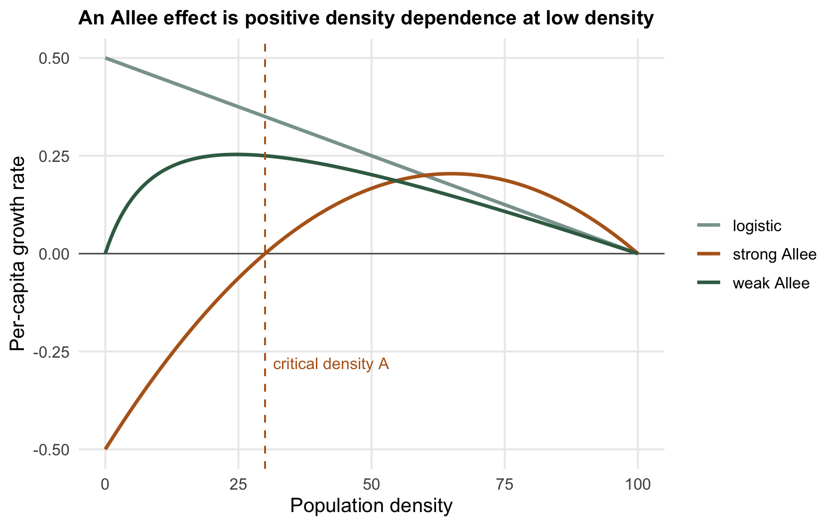
There are two flavours, and the difference is a matter of sign. Under a **weak** Allee effect per-capita growth is reduced when the population is sparse but stays positive: a rare population grows slowly, but it still grows. Under a **strong** Allee effect per-capita growth goes *negative* below a critical density: a population that falls below it shrinks to extinction on its own. That critical density is the whole story, so it is worth building all three per-capita growth curves side by side.
```{r curves}
r <- 0.5; K <- 100; A <- 30
g_log    <- function(N) r*(1 - N/K)                 # logistic: crowding only
g_weak   <- function(N) r*(1 - N/K)*(N/(N + 12))    # weak Allee: reduced but positive
g_strong <- function(N) r*(1 - N/K)*(N/A - 1)       # strong Allee: negative below A
sapply(list(logistic = g_log, weak = g_weak, strong = g_strong), function(f) f(10))
```
At a density of 10 the logistic population still grows at `r sprintf("%.2f", g_log(10))` per head, the weak-Allee one at a reduced but positive `r sprintf("%.2f", g_weak(10))`, and the strong-Allee one at `r sprintf("%.2f", g_strong(10))`: negative. Only the strong Allee effect has a density below which the population is doomed.
```{r fig-percap}
#| fig-cap: "Per-capita growth against density. The logistic line (grey) falls steadily. The weak Allee curve (green) drops towards zero as density approaches zero but never goes below it. The strong Allee curve (ochre) crosses zero at the critical density and is negative below it."
#| fig-alt: "Three per-capita growth curves against density; the grey logistic declines linearly, the green weak-Allee curve drops to zero at the origin but never goes below it, the ochre strong-Allee curve is negative below a critical density and positive above it."
Ng <- seq(0, 100, 0.5)
d <- rbind(data.frame(N = Ng, g = g_log(Ng),    type = "logistic"),
           data.frame(N = Ng, g = g_weak(Ng),   type = "weak Allee"),
           data.frame(N = Ng, g = g_strong(Ng), type = "strong Allee"))
ggplot(d, aes(N, g, colour = type)) +
  geom_hline(yintercept = 0, colour = col_ref, linewidth = 0.4) +
  geom_line(linewidth = 1) +
  geom_vline(xintercept = A, colour = col_strong, linetype = "dashed") +
  annotate("text", x = A + 1.5, y = -0.28, label = "critical density A", hjust = 0, colour = col_strong, size = 3.4) +
  scale_colour_manual(values = c("logistic" = col_log, "weak Allee" = col_weak, "strong Allee" = col_strong)) +
  labs(x = "Population density", y = "Per-capita growth rate", colour = NULL,
       title = "An Allee effect is positive density dependence at low density")
```
## The threshold is an unstable equilibrium
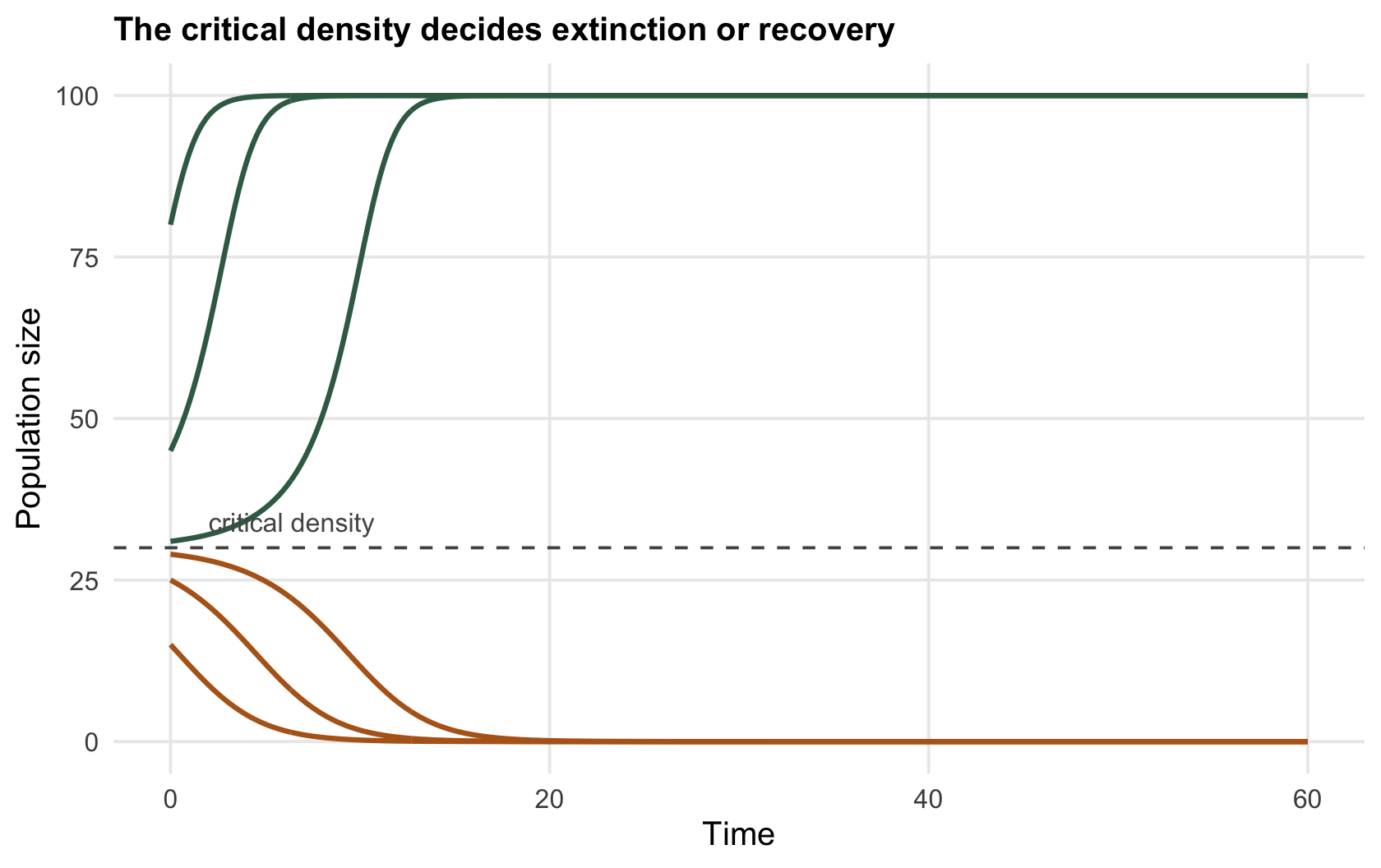
The strong Allee model has three equilibria: extinction at zero, carrying capacity at `r sprintf("%.0f", K)`, and the critical density at `r sprintf("%.0f", A)`. The first two are stable, attractors the population settles into. The critical density is *unstable*: it is a watershed, and the smallest push to either side sends the population away from it, up to carrying capacity or down to nothing. Run trajectories from just below and just above it.
```{r trajectories}
traj <- function(N0, g, tmax = 60, dt = 0.05) {
  N <- N0; out <- numeric(tmax/dt + 1); out[1] <- N0
  for (i in 2:length(out)) { N <- max(N + N*g(N)*dt, 0); out[i] <- N }
  data.frame(t = seq(0, tmax, dt), N = out)
}
sapply(c(25, 31), function(N0) round(tail(traj(N0, g_strong)$N, 1), 1))
```
A population starting at `r sprintf("%.0f", 25)`, five below the threshold, collapses to `r sprintf("%.1f", end_state[1])`. One starting at `r sprintf("%.0f", 31)`, one above it, climbs to `r sprintf("%.0f", end_state[2])`. Six individuals of difference in starting size decide extinction versus a full population. Nothing about the two populations differs except which side of the watershed they began on.
```{r fig-traj}
#| fig-cap: "Trajectories of a strong-Allee population from several starting sizes. Those below the critical density (dashed) fall to extinction; those above it rise to carrying capacity. The threshold divides the outcomes."
#| fig-alt: "Population trajectories over time from different starting sizes; curves starting below a dashed threshold line decline to zero, curves starting above it rise to carrying capacity."
runs <- do.call(rbind, lapply(c(15, 25, 29, 31, 45, 80), function(N0) {
  tr <- traj(N0, g_strong); tr$N0 <- factor(N0); tr }))
ggplot(runs, aes(t, N, group = N0, colour = N < 1 | N0 %in% c("15","25","29"))) +
  geom_hline(yintercept = A, colour = col_ref, linetype = "dashed") +
  geom_line(linewidth = 0.9) +
  annotate("text", x = 40, y = A + 4, label = "critical density", hjust = 0, colour = col_ref, size = 3.4) +
  scale_colour_manual(values = c("FALSE" = col_weak, "TRUE" = col_strong), guide = "none") +
  labs(x = "Time", y = "Population size", title = "The critical density decides extinction or recovery")
```
## Why the threshold is only the beginning
A deterministic threshold is a clean line, and reality is not. A real population does not sit at a fixed density and wait; it fluctuates, and near the threshold a run of bad luck can carry it across even when the average trend is upward. That is why a strong Allee effect makes extinction likely at densities the deterministic model calls safe, the subject of the [extinction-risk post](../allee-effects-and-extinction-risk/). Before that, the next post asks where the threshold comes from: an Allee effect at the population level is built from Allee effects on individual fitness components, and the two are not the same thing. And the threshold that matters most is the one hardest to see, because it lives at low density where populations are rare and data are thin, which the [checking post](../checking-an-allee-analysis/) takes up.
## References
- Courchamp F et al. 1999. Trends in Ecology and Evolution 14(10):405-410 (10.1016/S0169-5347(99)01683-3).
- Stephens PA, Sutherland WJ 1999. Trends in Ecology and Evolution 14(10):401-405 (10.1016/S0169-5347(99)01684-5).
- Stephens PA, Sutherland WJ, Freckleton RP 1999. Oikos 87(1):185-190 (10.2307/3547011).
## Related tutorials
- [Component and demographic Allee effects](../component-vs-demographic-allee/)
- [Allee effects and extinction risk](../allee-effects-and-extinction-risk/)
- [Checking an Allee analysis](../checking-an-allee-analysis/)
- [The theta-logistic model](../theta-logistic-model/)