---
title: "Component and demographic Allee effects"
description: "Component versus demographic Allee effects in R: how a mate-finding shortfall at low density scales up to a population threshold, and when it stays harmless."
date: "2026-07-01 11:00"
date-modified: "2026-10-07"
categories: [ecology tutorial, R, population ecology, behaviour, conservation]
image: thumbnail.png
image-alt: "A single orange curve of demographic critical density against mate-finding difficulty, near zero at a difficulty of one, about eight at twenty and twenty three at forty, then steepening sharply to about fifty at the right-hand end. The curve stays positive across the whole range and never crosses zero."
---
*Corrected 7 October 2026: the post said a component Allee effect becomes a population-level threshold only if it is strong enough; in this model even easy mate-finding leaves a threshold, a negligibly small one, so strength decides whether the threshold is large enough to matter, as the text and the plot title now say.*
```{r setup}
#| code-fold: true
#| code-summary: "Setup: packages, colours and plot theme"
#| results: hide
#| message: false
#| warning: false
knitr::opts_chunk$set(echo = TRUE, message = FALSE, warning = FALSE,
                      dev = "png", dpi = 120, fig.path = "figures/",
                      fig.width = 7, fig.height = 4.4)
library(ggplot2)
theme_te <- theme_minimal(base_size = 12) +
  theme(panel.background = element_rect(fill = "#f5f4ee", colour = NA),
        plot.background  = element_rect(fill = "#f5f4ee", colour = NA),
        panel.grid.minor = element_blank(),
        plot.title = element_text(face = "bold", size = 12))
theme_set(theme_te)
col_easy <- "#3a6b52"; col_hard <- "#b5651d"; col_ref <- "#555555"

b <- 1.2; d <- 0.3; a <- 0.006
mate <- function(N, theta) N/(N + theta)                  # component Allee: mate-finding
rN   <- function(N, theta) b*mate(N, theta) - d - a*N     # demographic per-capita growth
thresh <- function(theta) { Ng <- seq(0.05, 120, 0.05); up <- Ng[which(diff(sign(rN(Ng, theta))) > 0)]; if (length(up)) up[1] else NA }
A_easy <- thresh(2); A_hard <- thresh(30)
```
The [previous post](../allee-effects-and-thresholds/) treated the Allee effect as a property of a whole population: per-capita growth turning negative below a critical density. But populations do not have mating problems; individuals do. An Allee effect at the population level is assembled from Allee effects on the pieces of individual fitness, and the translation from one to the other is not automatic. Keeping the two levels apart is the point of this post (Stephens, Sutherland and Freckleton 1999 Oikos 87(1):185-190).
## Two levels
A **component** Allee effect is positive density dependence in a single component of fitness: the chance of finding a mate, the success of fertilisation, the effectiveness of group defence or cooperative hunting. A **demographic** Allee effect is positive density dependence in the bottom line, the per-capita growth rate of the whole population. The first is about one part of an individual's life; the second is about whether the population grows.
Build a demographic rate from a component. Let the component be mate-finding: the probability that a female finds a mate rises with density as `N/(N + theta)`, where `theta` sets how hard mates are to find. Births are this probability times a maximum rate, and against them stand a density-independent death rate and ordinary crowding.
```{r model}
b <- 1.2; d <- 0.3; a <- 0.006
mate <- function(N, theta) N/(N + theta)                 # the component Allee effect
rN   <- function(N, theta) b*mate(N, theta) - d - a*N    # the demographic growth rate
```
## The same component, two outcomes
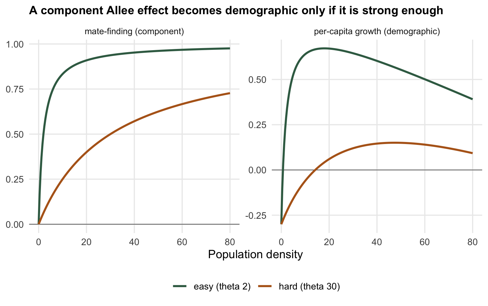
The mate-finding curve is a component Allee effect for any positive `theta`: it always rises with density. What it does to the population depends on how strong it is. Compare mates that are easy to find (`theta = 2`, the curve saturates almost at once) with mates that are hard (`theta = 30`, it climbs slowly).
```{r outcomes}
rbind(easy_theta2  = round(rN(c(2, 10, 40), 2), 3),
      hard_theta30 = round(rN(c(2, 10, 40), 30), 3))
```
When mates are easy to find, per-capita growth is already positive at a density of `r sprintf("%.0f", 2)` and there is no meaningful threshold: the demographic Allee effect exists in principle but its critical density sits near `r sprintf("%.1f", A_easy)`, below one individual, of no consequence to a real population. When mates are hard to find, per-capita growth is negative up to a critical density of `r sprintf("%.1f", A_hard)`, a strong demographic Allee effect at a density a population can easily fall to. The component was the same kind of thing in both cases. Only its strength decided whether the population-level threshold it produced was large enough to matter.
```{r fig-mate}
#| fig-cap: "The mate-finding component (left) rises with density for both parameter values; the demographic growth it produces (right) crosses zero at a density worth worrying about only when mates are hard to find."
#| fig-alt: "Two panels: on the left, two rising mate-finding curves; on the right, the per-capita growth curves they produce, both starting below zero: one crossing zero almost at once, the other staying negative until a density of about 14."
Ng <- seq(0, 80, 0.4)
comp <- rbind(data.frame(N = Ng, y = mate(Ng, 2),  theta = "easy (theta 2)",  panel = "mate-finding (component)"),
              data.frame(N = Ng, y = mate(Ng, 30), theta = "hard (theta 30)", panel = "mate-finding (component)"))
demo <- rbind(data.frame(N = Ng, y = rN(Ng, 2),  theta = "easy (theta 2)",  panel = "per-capita growth (demographic)"),
              data.frame(N = Ng, y = rN(Ng, 30), theta = "hard (theta 30)", panel = "per-capita growth (demographic)"))
both <- rbind(comp, demo)
ggplot(both, aes(N, y, colour = theta)) +
  geom_hline(yintercept = 0, colour = col_ref, linewidth = 0.3) +
  geom_line(linewidth = 1) +
  facet_wrap(~panel, scales = "free_y") +
  scale_colour_manual(values = c("easy (theta 2)" = col_easy, "hard (theta 30)" = col_hard)) +
  labs(x = "Population density", y = NULL, colour = NULL,
       title = "A component Allee effect sets a threshold that matters only if it is strong") +
  theme(strip.text = element_text(size = 9), legend.position = "bottom")
```
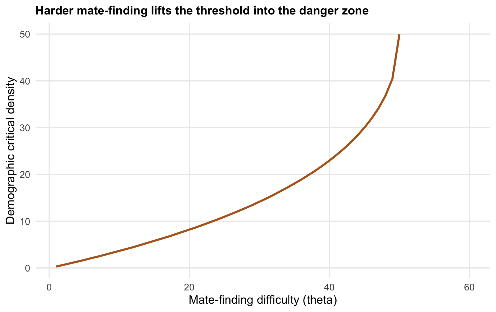
There is a continuum between these two cases. As mates get harder to find, the demographic threshold climbs from a harmless fraction of an individual to a density that dominates the population's fate.
```{r fig-threshold}
#| fig-cap: "The demographic critical density against how hard mates are to find. Below a mild difficulty the threshold is negligible; past it, the threshold rises steeply into the range a real population occupies. The line stops at a difficulty of 50, where the threshold ceases to exist."
#| fig-alt: "A rising curve of critical density against the mate-finding difficulty parameter, near zero at low difficulty and climbing steeply as mates become harder to find, ending abruptly about five sixths of the way along the axis."
th <- seq(1, 60, 1)
dt <- data.frame(theta = th, A = sapply(th, thresh))
ggplot(dt, aes(theta, A)) +
  geom_line(colour = col_hard, linewidth = 1) +
  labs(x = "Mate-finding difficulty (theta)", y = "Demographic critical density",
       title = "Harder mate-finding lifts the threshold into the danger zone")
```
The line ends at a difficulty of 50 rather than at the edge of the plot, and that gap is the result, not a plotting fault. Past that point per-capita growth is negative at every density: the population cannot grow from any starting size, so there is no critical density to cross, `thresh` returns `NA` and the ten remaining points are dropped from the figure.
## Why the distinction earns its keep
Two practical consequences follow. First, a component Allee effect can be masked. If low density relaxes some other limit, less competition for food, fewer shared parasites, the gain can offset the mating shortfall, and a population showing a clear mate-finding problem can still have no demographic Allee effect at all (Stephens et al. 1999; Courchamp et al. 1999 Trends in Ecology and Evolution 14(10):405-410). Measuring the component alone can therefore mislead about the population. Second, the reverse: a demographic Allee effect can be built from several weak components, none alarming on its own, that stack. Mate limitation plus weaker group defence plus reduced foraging efficiency can together push per-capita growth negative where no single one would.
So the component is where the mechanism lives and the demographic rate is where the consequence lives, and conservation needs both: the mechanism to know what to fix, the demographic rate to know whether fixing it matters. The [extinction-risk post](../allee-effects-and-extinction-risk/) takes the demographic threshold into a fluctuating world, where it does its real damage.
## References
- Courchamp F et al. 1999. Trends in Ecology and Evolution 14(10):405-410 (10.1016/S0169-5347(99)01683-3).
- Kramer AM et al. 2009. Population Ecology 51(3):341-354 (10.1007/s10144-009-0152-6).
- Stephens PA, Sutherland WJ, Freckleton RP 1999. Oikos 87(1):185-190 (10.2307/3547011).
## Related tutorials
- [Allee effects and thresholds in R](../allee-effects-and-thresholds/)
- [Allee effects and extinction risk](../allee-effects-and-extinction-risk/)
- [Checking an Allee analysis](../checking-an-allee-analysis/)
- [GLM for count data and abundance](../glm-count-data-abundance/)