---
title: "Checking an Allee analysis"
description: "Three checks for an Allee effect in R: why detection needs low-density data, how sampling error fakes density dependence, and strong versus weak Allee."
date: "2026-07-01 12:00"
date-modified: "2026-10-15"
categories: [ecology tutorial, R, population ecology, model diagnostics, conservation]
image: thumbnail.png
image-alt: "Per-capita growth against density where a positive low-density trend reveals an Allee effect that a high-density-only fit would miss."
---
*Corrected 15 October 2026: the first check explained the nearly flat high-density fit by the line averaging the end of the rise with the decline beyond it; a straight line through the model's own curve over those densities slopes down, so the text now says the flat fit is a feature of this sample.*
*Corrected 7 October 2026: the first check said the Allee signature lives only below the critical threshold and that the high-density fit slopes the ordinary way, downward; in the post's own model per-capita growth keeps rising well above the threshold, so the text, the figure title, caption and alt text now say the signal is clearest at low density and that a straight line through the high-density data is nearly flat, because it spans the end of the rise and the decline beyond it.*
*Corrected 30 September 2026: the post said measurement error can hide or fake an Allee effect; the artefact shown always pushes the slope down, so it can mask an Allee effect but not create one, and both passages now say so.*
```{r setup}
#| code-fold: true
#| code-summary: "Setup: packages, colours and plot theme"
#| results: hide
#| message: false
#| warning: false
knitr::opts_chunk$set(echo = TRUE, message = FALSE, warning = FALSE,
                      dev = "png", dpi = 120, fig.path = "figures/",
                      fig.width = 7, fig.height = 4.4)
library(ggplot2)
theme_te <- theme_minimal(base_size = 12) +
  theme(panel.background = element_rect(fill = "#f5f4ee", colour = NA),
        plot.background  = element_rect(fill = "#f5f4ee", colour = NA),
        panel.grid.minor = element_blank(),
        plot.title = element_text(face = "bold", size = 12))
theme_set(theme_te)
col_lo <- "#b5651d"; col_hi <- "#3a6b52"; col_ref <- "#555555"

r <- 0.5; K <- 100; A <- 30
pgr <- function(N) r*(1 - N/K)*(N/A - 1)
set.seed(4021)
Nobs <- runif(80, 5, 100); pc <- pgr(Nobs) + rnorm(80, 0, 0.07)
fit_hi <- lm(pc ~ Nobs, subset = Nobs > 40); fit_lo <- lm(pc ~ Nobs, subset = Nobs < A)
sl_hi <- coef(fit_hi)[2]; sl_lo <- coef(fit_lo)[2]
p_hi <- summary(fit_hi)$coefficients[2, 4]; p_lo <- summary(fit_lo)$coefficients[2, 4]

## measurement error fakes density dependence
set.seed(402)
Tn <- 200; Ntrue <- numeric(Tn); Ntrue[1] <- 60
for (t in 2:Tn) Ntrue[t] <- Ntrue[t-1]*exp(rnorm(1, 0, 0.10))   # density-INDEPENDENT truth
obs <- Ntrue*exp(rnorm(Tn, 0, 0.25))
sl_true <- coef(lm(diff(log(Ntrue)) ~ Ntrue[-Tn]))[2]
sl_err  <- coef(lm(diff(log(obs))  ~ obs[-Tn]))[2]
```
```{r sci-tex-helper}
#| include: false
sci_tex <- function(x, digits = 2) {
s <- formatC(x, format = "e", digits = digits)
paste0("$", sub("e.*", "", s), " \\times 10^{", as.integer(sub(".*e", "", s)), "}$")
}
```
An Allee effect is easy to propose and hard to prove. The mechanism is plausible for almost any species, mates get scarce, groups get too small, and the consequences for conservation are serious, so the temptation is to assume one is present. The evidence base is much thinner than the literature's attention would suggest (Kramer et al. 2009 Population Ecology 51(3):341-354), and the reasons are three specific problems that any analysis should confront.
## Check 1: is there any low-density data?
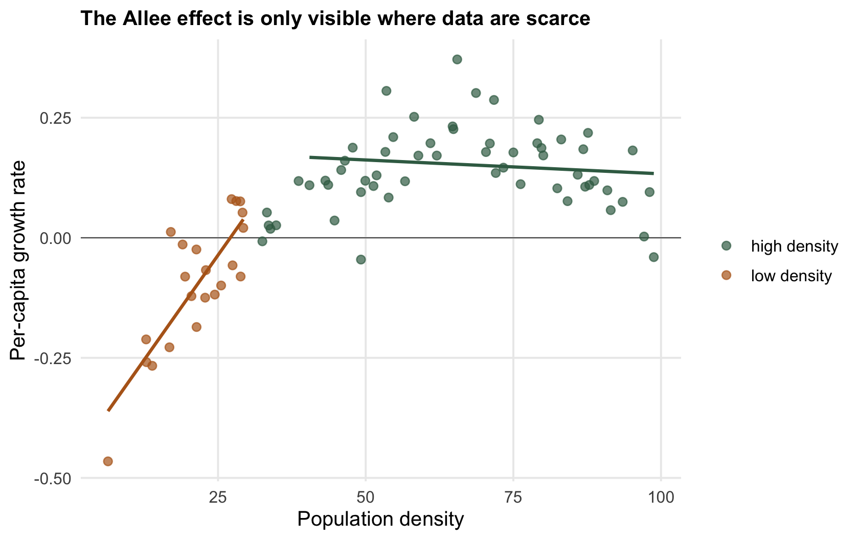
The Allee signature is positive density dependence: per-capita growth rising with density. It is clearest at low density, below the [critical threshold](../allee-effects-and-thresholds/), where growth is negative, but it does not stop there: in the model below per-capita growth keeps rising up to a density of `r sprintf("%.0f", (A + K) / 2)` before crowding takes over. Fit per-capita growth against density using only the densities a healthy population occupies and you will find a flat or downward slope and conclude there is no Allee effect, when the whole point is what happens below where you looked.
```{r detection}
r <- 0.5; K <- 100; A <- 30
pgr <- function(N) r*(1 - N/K)*(N/A - 1)              # the true dynamics have a strong Allee effect
Ng <- seq(40, 100, by = 0.5); sl_model <- coef(lm(pgr(Ng) ~ Ng))[2]   # straight line through the true curve above 40
rbind(high_density = c(slope = unname(sl_hi), p = unname(p_hi)),
      low_density  = c(slope = unname(sl_lo), p = unname(p_lo)))
```
Fitted on densities above `r sprintf("%.0f", 40)`, per-capita growth has a slope of `r sprintf("%.4f", sl_hi)` with p = `r sprintf("%.2f", p_hi)`: in this sample a straight line through the high-density data is nearly flat, although the same fit to the model's own curve over these densities slopes down at `r sprintf("%.4f", sl_model)`, since the crowding decline beyond the peak outweighs the end of the rise. Flat or downward, on that fit alone nothing points to an Allee effect. Fitted on densities below the threshold of `r sprintf("%.0f", A)`, it slopes *up* at `r sprintf("%.4f", sl_lo)` and this one is unambiguous (p = `r sci_tex(p_lo, 1)`), the Allee signature. Same population, opposite conclusions, decided entirely by which densities were sampled. The cruelty of it is that the low densities are exactly the hardest to observe: a population rare enough to be in Allee territory is rare enough to be hard to find and count.
```{r fig-detect}
#| fig-cap: "Per-capita growth against density for a population with a strong Allee effect. The low-density points (ochre) trend upward, the Allee signature; a straight-line fit to the upper part of the high-density range alone (green line) is nearly flat and misses it entirely."
#| fig-alt: "Scatter of per-capita growth against density with two fitted lines; the low-density line slopes up while the high-density line is nearly flat, showing that the Allee effect is missed when only the high densities are fitted."
dd <- data.frame(N = Nobs, pc = pc, band = ifelse(Nobs < A, "low density", "high density"))
ggplot(dd, aes(N, pc)) +
  geom_hline(yintercept = 0, colour = col_ref, linewidth = 0.3) +
  geom_point(aes(colour = band), size = 2, alpha = 0.7) +
  geom_smooth(data = subset(dd, N < A), method = "lm", se = FALSE, colour = col_lo, linewidth = 0.9) +
  geom_smooth(data = subset(dd, N > 40), method = "lm", se = FALSE, colour = col_hi, linewidth = 0.9) +
  scale_colour_manual(values = c("low density" = col_lo, "high density" = col_hi)) +
  labs(x = "Population density", y = "Per-capita growth rate", colour = NULL,
       title = "The Allee effect is clearest where data are scarce")
```
## Check 2: is the density dependence real or a measurement artefact?
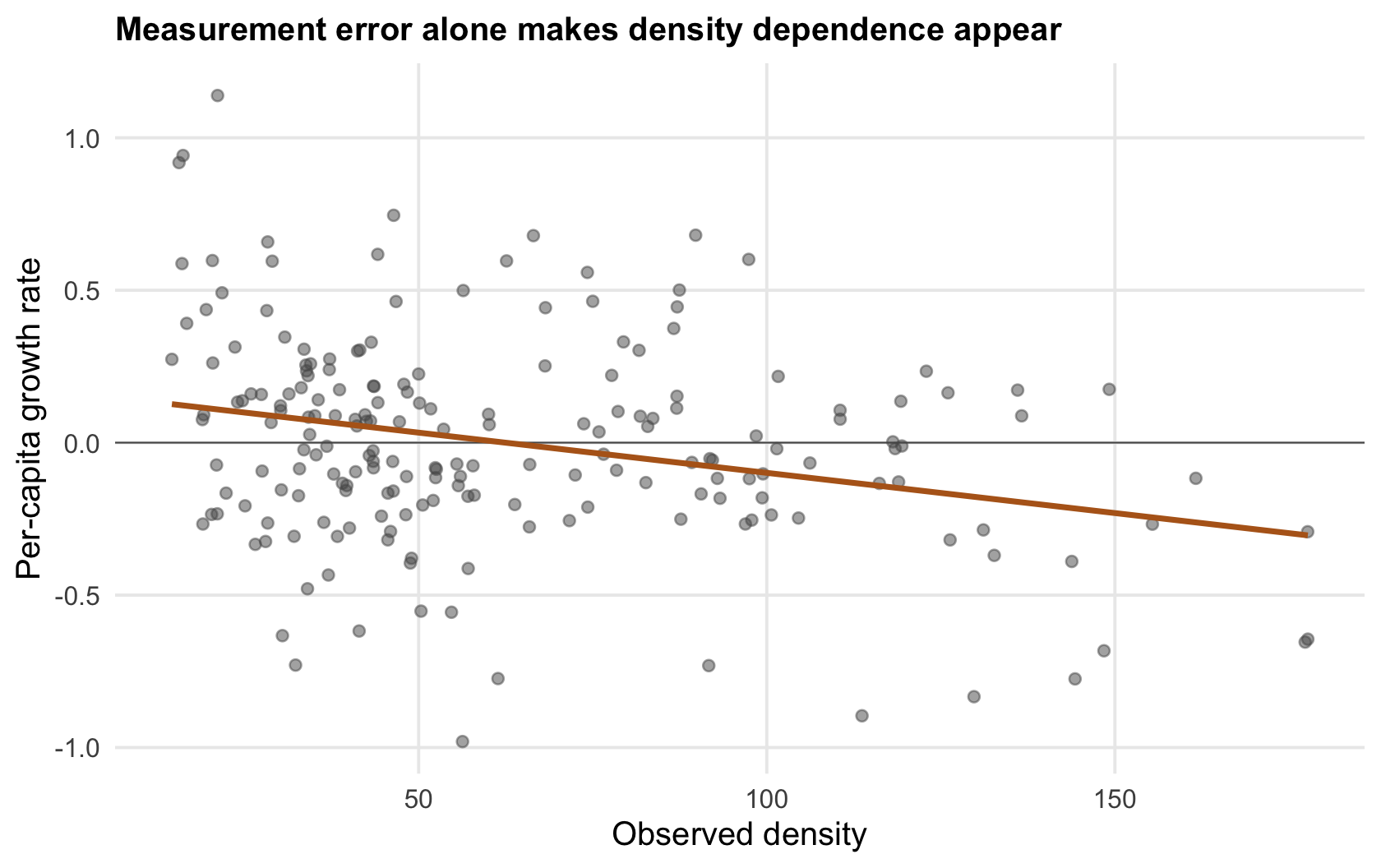
Suppose you do have counts across a range of densities. Counts are estimates, and estimates carry error, and error alone manufactures density dependence through regression to the mean. A year whose count happens to be over-estimated is usually followed by a lower count, not because the population declined but because the next estimate is closer to the truth. That looks exactly like decline following high density.
```{r regmean}
set.seed(402)
Ntrue <- 60; for (t in 2:200) Ntrue[t] <- Ntrue[t-1]*exp(rnorm(1, 0, 0.10))  # NO density dependence
obs <- Ntrue*exp(rnorm(200, 0, 0.25))                                        # counts with 25% error
c(slope_true_N = unname(sl_true), slope_observed_N = unname(sl_err))
```
The true dynamics here are density-independent, a random walk: the slope of growth on the true density is `r sprintf("%.4f", sl_true)`, indistinguishable from zero. Recompute growth from the *observed* counts, regress that on observed density, and the slope is `r sprintf("%.4f", sl_err)`, an order of magnitude larger and firmly negative. Both axes are now built from the same noisy counts: an over-estimate raises the density on the x axis and depresses the growth on the y axis, so density dependence appears with no change at all in the dynamics. Because the artefact always pushes the slope down, the same mechanism can hide a real Allee effect, whose signature is an upward slope at low density. The check is to model the observation error, with a state-space model, or to use independent estimates for density and for growth so the error in one does not drive the other.
```{r fig-regmean}
#| fig-cap: "Regression to the mean. The population is density-independent, yet plotting growth against the error-laden count (points, ochre fit) produces a clear downward slope that is pure measurement artefact."
#| fig-alt: "Scatter of per-capita growth against observed density with a downward-sloping fitted line, despite the underlying dynamics having no density dependence."
dr <- data.frame(N = obs[-200], g = diff(log(obs)))
ggplot(dr, aes(N, g)) +
  geom_hline(yintercept = 0, colour = col_ref, linewidth = 0.3) +
  geom_point(colour = col_ref, size = 1.6, alpha = 0.5) +
  geom_smooth(method = "lm", se = FALSE, colour = col_lo, linewidth = 1) +
  labs(x = "Observed density", y = "Per-capita growth rate",
       title = "Measurement error alone makes density dependence appear")
```
## Check 3: strong, weak, or none?
Even with honest low-density data, the three cases that matter for conservation, a strong Allee effect with a threshold, a weak one without, and no Allee effect, are hard to separate, because they differ only in the sparse low-density region and the data there are few and noisy. A model can be fitted, but the confidence interval on the critical density is usually wide, often running down to zero, which means the data cannot rule out "no threshold". Report that interval honestly rather than a point estimate of the threshold, and resist reading a fitted `A` as if it were measured.
## The precautionary reading
These checks mostly deliver bad news: the effect is real in theory, hard to detect in practice, and easy to mask with noise. That asymmetry has a consequence for how the absence of evidence should be read. Failing to detect an Allee effect in a data set that never sampled low densities, or that carries ordinary counting error, is not evidence that none exists. For a species being managed down toward small numbers, the cost of wrongly assuming safety is extinction, and the cost of wrongly assuming a threshold is caution. The honest analysis states what the data can and cannot see, and where they cannot see, it errs toward the threshold being real.
## References
- Kramer AM et al. 2009. Population Ecology 51(3):341-354 (10.1007/s10144-009-0152-6).
- Stephens PA, Sutherland WJ, Freckleton RP 1999. Oikos 87(1):185-190 (10.2307/3547011).
- Taylor CM, Hastings A 2005. Ecology Letters 8(8):895-908 (10.1111/j.1461-0248.2005.00787.x).
## Related tutorials
- [Allee effects and thresholds in R](../allee-effects-and-thresholds/)
- [Component and demographic Allee effects](../component-vs-demographic-allee/)
- [Allee effects and extinction risk](../allee-effects-and-extinction-risk/)
- [Detecting density dependence](../detecting-density-dependence/)