---
title: "Allee effects and extinction risk"
description: "Allee effects and extinction risk in R: why demographic stochasticity endangers populations above the critical density, and why small introductions fail."
date: "2026-07-01 10:00"
categories: [ecology tutorial, R, population ecology, conservation, extinction]
image: thumbnail.png
image-alt: "Extinction probability against starting population size, high near the threshold for an Allee population and near zero for a population without one."
---
```{r setup}
#| code-fold: true
#| code-summary: "Setup: packages, colours, plot theme and the simulation grids behind both figures"
#| results: hide
#| message: false
#| warning: false
knitr::opts_chunk$set(echo = TRUE, message = FALSE, warning = FALSE,
                      dev = "png", dpi = 120, fig.path = "figures/",
                      fig.width = 7, fig.height = 4.4)
library(ggplot2)
theme_te <- theme_minimal(base_size = 12) +
  theme(panel.background = element_rect(fill = "#f5f4ee", colour = NA),
        plot.background  = element_rect(fill = "#f5f4ee", colour = NA),
        panel.grid.minor = element_blank(),
        plot.title = element_text(face = "bold", size = 12))
theme_set(theme_te)
col_allee <- "#b5651d"; col_no <- "#3a6b52"; col_ref <- "#555555"

r <- 0.5; K <- 100; A <- 30
step_pop <- function(N, allee) {
  g <- if (allee) r*(1 - N/K)*(N/A - 1) else r*(1 - N/K)
  rpois(1, N * exp(g))
}
sim_ext <- function(N0, allee, tmax = 100, reps = 600) {
  ext <- 0
  for (j in 1:reps) { N <- N0
    for (t in 1:tmax) { if (N < 1) { N <- 0; break }; N <- step_pop(N, allee); if (N < 1) { N <- 0; break } }
    if (N < 1) ext <- ext + 1 }
  ext/reps
}
sim_est <- function(N0, allee, tmax = 80, reps = 600) {
  est <- 0
  for (j in 1:reps) { N <- N0
    for (t in 1:tmax) { if (N < 1) { N <- 0; break }; N <- step_pop(N, allee); if (N < 1) { N <- 0; break } }
    if (N >= K/2) est <- est + 1 }
  est/reps
}
set.seed(401)
ext_grid <- data.frame(N0 = seq(30, 72, 3))
ext_grid$allee <- sapply(ext_grid$N0, sim_ext, allee = TRUE)
ext_grid$none  <- sapply(ext_grid$N0, sim_ext, allee = FALSE)
est_grid <- data.frame(N0 = seq(6, 60, 3))
est_grid$allee <- sapply(est_grid$N0, sim_est, allee = TRUE)
est_grid$none  <- sapply(est_grid$N0, sim_est, allee = FALSE)
```
The [critical density](../allee-effects-and-thresholds/) of a strong Allee effect is a clean line in a deterministic model: above it a population recovers, below it a population dies. Real populations do not read the model. They are made of individuals that are born and die by chance, and near a threshold that chance is decisive. This is where the Allee effect does its real harm, and it takes a stochastic simulation to see it.
## Stochasticity makes the threshold leak
Model the population in discrete steps with demographic stochasticity: each generation the next count is a Poisson draw around the expected growth. Run it many times from each starting size, once with a strong Allee effect and once without, and record how often the population is extinct after a century.
```{r sim}
r <- 0.5; K <- 100; A <- 30
step_pop <- function(N, allee) {
  g <- if (allee) r*(1 - N/K)*(N/A - 1) else r*(1 - N/K)   # strong Allee, or plain logistic
  rpois(1, N * exp(g))                                      # demographic stochasticity
}
sim_ext <- function(N0, allee, tmax = 100, reps = 600) {     # extinct after tmax steps?
  ext <- 0
  for (j in 1:reps) { N <- N0
    for (t in 1:tmax) { if (N < 1) { N <- 0; break }; N <- step_pop(N, allee); if (N < 1) { N <- 0; break } }
    if (N < 1) ext <- ext + 1 }
  ext/reps
}
sim_est <- function(N0, allee, tmax = 80, reps = 600) {      # reached half of K?
  est <- 0
  for (j in 1:reps) { N <- N0
    for (t in 1:tmax) { if (N < 1) { N <- 0; break }; N <- step_pop(N, allee); if (N < 1) { N <- 0; break } }
    if (N >= K/2) est <- est + 1 }
  est/reps
}
set.seed(401)
ext36 <- c(allee_from_36 = sim_ext(36, TRUE), logistic_from_36 = sim_ext(36, FALSE))
ext36
```
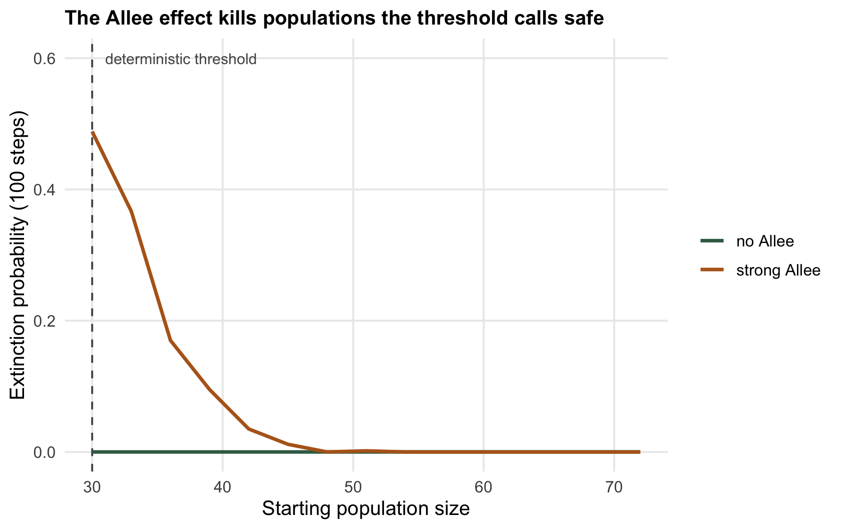
A population of `r sprintf("%.0f", 36)`, a fifth above the deterministic threshold of `r sprintf("%.0f", A)`, has a `r sprintf("%.0f", 100 * ext36[["allee_from_36"]])` per cent chance of extinction within a century when it carries a strong Allee effect. The curve below, built from a separate set of runs, puts the same starting size at `r sprintf("%.0f", 100 * ext_grid$allee[ext_grid$N0 == 36])` per cent, which is the Monte Carlo error to expect from 600 replicates. The same population under ordinary crowding, no Allee effect, essentially never goes extinct. The deterministic model called `r sprintf("%.0f", 36)` safe; stochastically it is not, because a run of chance shortfalls in births and survival can push the count below the threshold, and once below, the Allee effect finishes the job.
```{r fig-ext}
#| fig-cap: "Extinction probability against starting size. Without an Allee effect (green) even small populations persist. With a strong Allee effect (ochre) the risk stays high well above the deterministic threshold (dashed) and only fades as the population clears it with room to spare."
#| fig-alt: "Two curves of extinction probability against starting population size; the green no-Allee curve is near zero throughout, the ochre Allee curve is high near the threshold and declines as starting size grows."
el <- rbind(data.frame(N0 = ext_grid$N0, p = ext_grid$allee, type = "strong Allee"),
            data.frame(N0 = ext_grid$N0, p = ext_grid$none,  type = "no Allee"))
ggplot(el, aes(N0, p, colour = type)) +
  geom_vline(xintercept = A, colour = col_ref, linetype = "dashed") +
  geom_line(linewidth = 1) +
  annotate("text", x = A + 1, y = 0.6, label = "deterministic threshold", hjust = 0, colour = col_ref, size = 3.2) +
  scale_colour_manual(values = c("strong Allee" = col_allee, "no Allee" = col_no)) +
  labs(x = "Starting population size", y = "Extinction probability (100 steps)", colour = NULL,
       title = "The Allee effect kills populations the threshold calls safe")
```
## Why small introductions fail
The same logic runs in reverse for a population starting from scratch: a colonising propagule, a reintroduction, an invasive species arriving in a new range. It begins small, exactly where the Allee effect bites. Ask how often a release establishes, reaching a viable size, as a function of how many individuals are released.
```{r establishment}
set.seed(401)
est_out <- c(released_12 = sim_est(12, TRUE), released_42 = sim_est(42, TRUE),
             released_12_noallee = sim_est(12, FALSE))
est_out
```
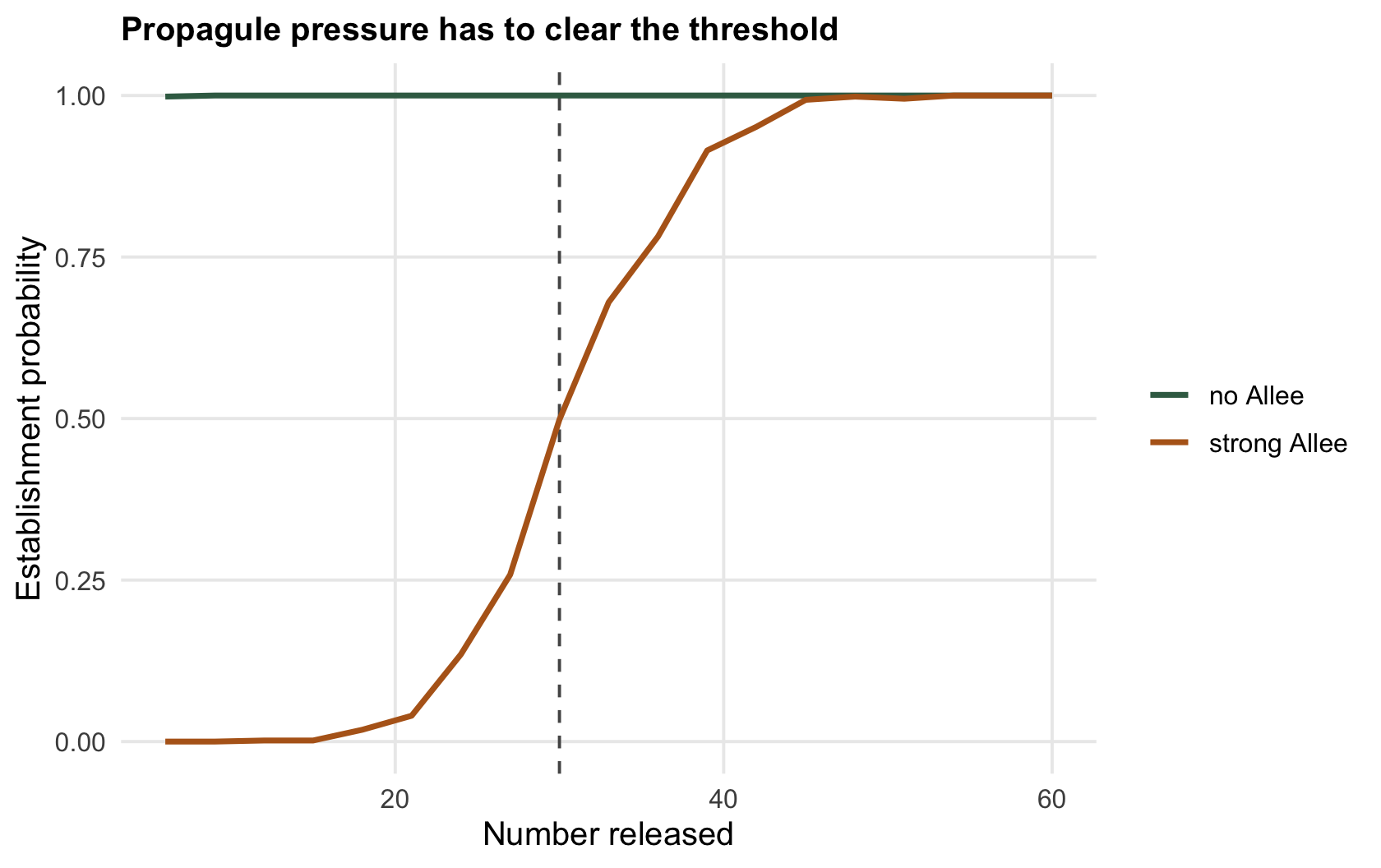
With a strong Allee effect, releasing `r sprintf("%.0f", 12)` individuals established a population in none of the `r 600` runs, so the honest reading is essentially never rather than never; releasing `r sprintf("%.0f", 42)` succeeds `r sprintf("%.0f", 100 * est_out[["released_42"]])` per cent of the time. Without the Allee effect a dozen individuals is already almost certain to take. The Allee effect turns establishment into a numbers game with a threshold: propagule pressure, the size and frequency of releases, becomes the thing that decides success (Taylor and Hastings 2005 Ecology Letters 8(8):895-908). It is why reintroductions are done in large cohorts, and why a handful of escaped invaders often fizzles while a large introduction takes hold.
```{r fig-est}
#| fig-cap: "Establishment probability against the number released. With a strong Allee effect (ochre) release must clear the threshold, and the curve is S-shaped; without one (green) even a few individuals establish."
#| fig-alt: "Two curves of establishment probability against number released; the ochre Allee curve rises steeply through an S-shape near the threshold, the green no-Allee curve is high from the smallest releases."
sl <- rbind(data.frame(N0 = est_grid$N0, p = est_grid$allee, type = "strong Allee"),
            data.frame(N0 = est_grid$N0, p = est_grid$none,  type = "no Allee"))
ggplot(sl, aes(N0, p, colour = type)) +
  geom_vline(xintercept = A, colour = col_ref, linetype = "dashed") +
  geom_line(linewidth = 1) +
  scale_colour_manual(values = c("strong Allee" = col_allee, "no Allee" = col_no)) +
  labs(x = "Number released", y = "Establishment probability", colour = NULL,
       title = "Propagule pressure has to clear the threshold")
```
## One accelerant among several
An Allee effect is a powerful way to turn a small population into no population, but it is not the only one, and honest risk assessment keeps them in view together. Environmental stochasticity, bad years that hit every individual at once, adds variance the demographic model here leaves out. Small populations also lose genetic variation and suffer inbreeding, a slower drain that compounds the demographic one. Habitat loss sets the stage for all of it. The Allee effect belongs in that list as an accelerant: it steepens the last stretch of decline and raises the size a population needs to be safe. Quantifying it for a real species is the hard part, because the threshold sits at low density where data are thinnest; that is the subject of the [checking post](../checking-an-allee-analysis/).
## References
- Kramer AM et al. 2009. Population Ecology 51(3):341-354 (10.1007/s10144-009-0152-6).
- Stephens PA, Sutherland WJ 1999. Trends in Ecology and Evolution 14(10):401-405 (10.1016/S0169-5347(99)01684-5).
- Taylor CM, Hastings A 2005. Ecology Letters 8(8):895-908 (10.1111/j.1461-0248.2005.00787.x).
## Related tutorials
- [Allee effects and thresholds in R](../allee-effects-and-thresholds/)
- [Component and demographic Allee effects](../component-vs-demographic-allee/)
- [Checking an Allee analysis](../checking-an-allee-analysis/)
- [Extinction risk and population viability analysis](../extinction-risk-pva/)