The theta-logistic model in R

Fitting the theta-logistic population growth model in R by maximum likelihood, and why the shape parameter theta is barely identifiable from one time series.

The logistic model assumes that per-capita growth falls in a straight line as a population fills up. The theta-logistic relaxes that assumption with one extra exponent, letting the braking be gentle at low density and sudden near the ceiling, or the reverse. It is a popular way to ask what shape density dependence takes. The catch is that the shape parameter is one of the hardest quantities in population ecology to estimate: a single time series usually cannot tell a gentle curve from a sharp one. This post fits the theta-logistic in base R by maximum likelihood and then shows, with a profile likelihood, why the shape parameter should be treated with suspicion.

The model and the shape parameter

On the log scale the theta-logistic writes the population growth rate as a function of density:

\[N_{t+1} = N_t \exp\!\big[\,r\,(1 - (N_t/K)^{\theta}) + \varepsilon_t\,\big], \qquad \varepsilon_t \sim \mathrm{Normal}(0, \sigma^2).\]

The exponent \(\theta\) sets the shape. With \(\theta = 1\) the growth rate falls linearly with density, the discrete logistic or Ricker form. With \(\theta\) below one the braking acts mostly at low density; with \(\theta\) above one the population grows almost unchecked until it nears \(K\) and then brakes hard. The trouble is already visible in the equation. Near \(K\) the term \(1 - (N/K)^{\theta}\) is close to zero for every \(\theta\), so the shape only shows itself when the population sits well below \(K\). A series that spends most of its time near carrying capacity carries almost no information about \(\theta\).

sim_theta <- function(T,r,K,theta,sigma,N1){ N<-numeric(T); N[1]<-N1
  for(t in 1:(T-1)){ pgr<-r*(1-(N[t]/K)^theta)+rnorm(1,0,sigma)
    N[t+1]<-N[t]*exp(pgr); if(N[t+1]<1) N[t+1]<-1 }
  N }
## process-only negative log-likelihood (sigma profiled out); optional fixed theta
nll <- function(par, pgr, dens, theta_fix=NA){
  r<-exp(par[1]); K<-exp(par[2]); theta<-if(is.na(theta_fix)) exp(par[3]) else theta_fix
  mu<-r*(1-(dens/K)^theta); s2<-mean((pgr-mu)^2); n<-length(pgr)
  0.5*n*(log(2*pi*s2)+1) }
fit_full <- function(N){ pgr<-diff(log(N)); dens<-N[-length(N)]
  op<-optim(c(log(0.3),log(max(N)*1.05),log(1)), nll, pgr=pgr, dens=dens,
            method="BFGS", control=list(maxit=2000))
  s2<-mean((pgr-exp(op$par[1])*(1-(dens/exp(op$par[2]))^exp(op$par[3])))^2)
  list(r=exp(op$par[1]), K=exp(op$par[2]), theta=exp(op$par[3]), sigma=sqrt(s2),
       ll=-op$value, conv=op$convergence) }
fit_theta <- function(N,theta){ pgr<-diff(log(N)); dens<-N[-length(N)]
  op<-optim(c(log(0.3),log(max(N)*1.05)), nll, pgr=pgr, dens=dens, theta_fix=theta,
            method="BFGS", control=list(maxit=2000))
  list(r=exp(op$par[1]), K=exp(op$par[2]), ll=-op$value) }

A series that reaches its ceiling

Simulate forty years from a theta-logistic with a true shape of \(\theta = 2.5\), starting at a quarter of carrying capacity so the population climbs and then settles near \(K = 1000\).

r_true<-0.40; K_true<-1000; theta_true<-2.5; sigma_true<-0.10; N1<-250; Tlen<-40
set.seed(12); N <- sim_theta(Tlen, r_true, K_true, theta_true, sigma_true, N1)

Fit the full four-parameter model by maximum likelihood. Because the growth-rate residuals are treated as Gaussian, this is a nonlinear least-squares fit of the growth rate on density, with the noise standard deviation falling out as the residual spread.

ff <- fit_full(N)
c(r=round(ff$r,2), K=round(ff$K,0), theta=round(ff$theta,2), sigma=round(ff$sigma,3))

      r       K   theta   sigma 
  0.390 995.000   1.780   0.083 

The fit recovers \(r\) as \(0.39\) and \(K\) as \(995\), both close to the true \(0.40\) and \(1000\). The shape parameter comes back as \(1.78\), already some way from the true \(2.5\), and that single point estimate hides how little the data pin it down. Two quite different shapes fit the same scatter almost equally well.

fR  <- fit_theta(N, 1)      # Ricker: theta fixed at 1
fHi <- fit_theta(N, 3.3)    # a sharply concave shape
c(ricker_ll=round(fR$ll,2), theta3.3_ll=round(fHi$ll,2), ml_ll=round(ff$ll,2),
  ricker_gap=round(ff$ll-fR$ll,2), theta3.3_gap=round(ff$ll-fHi$ll,2))

   ricker_ll  theta3.3_ll        ml_ll   ricker_gap theta3.3_gap 
       41.16        40.21        41.93         0.77         1.72 

pgr<-diff(log(N)); dens<-N[-length(N)]
gx <- seq(min(dens)*0.9, max(dens)*1.02, length.out=250)
curve_df <- rbind(
  data.frame(N=gx, pgr=fR$r*(1-(gx/fR$K)^1),    model="theta = 1 (Ricker)"),
  data.frame(N=gx, pgr=fHi$r*(1-(gx/fHi$K)^3.3), model="theta = 3.3"))
ggplot()+
  geom_hline(yintercept=0, colour=faint, linewidth=.3)+
  geom_point(data=data.frame(N=dens,pgr=pgr), aes(N, pgr), colour=ink, size=1.9, alpha=.8)+
  geom_line(data=curve_df, aes(N, pgr, colour=model), linewidth=1)+
  scale_colour_manual(values=c("theta = 1 (Ricker)"=forest,"theta = 3.3"=aban))+
  labs(x="density N", y="population growth rate", colour=NULL,
       title="Two very different shapes fit the same data")+
  theme_te()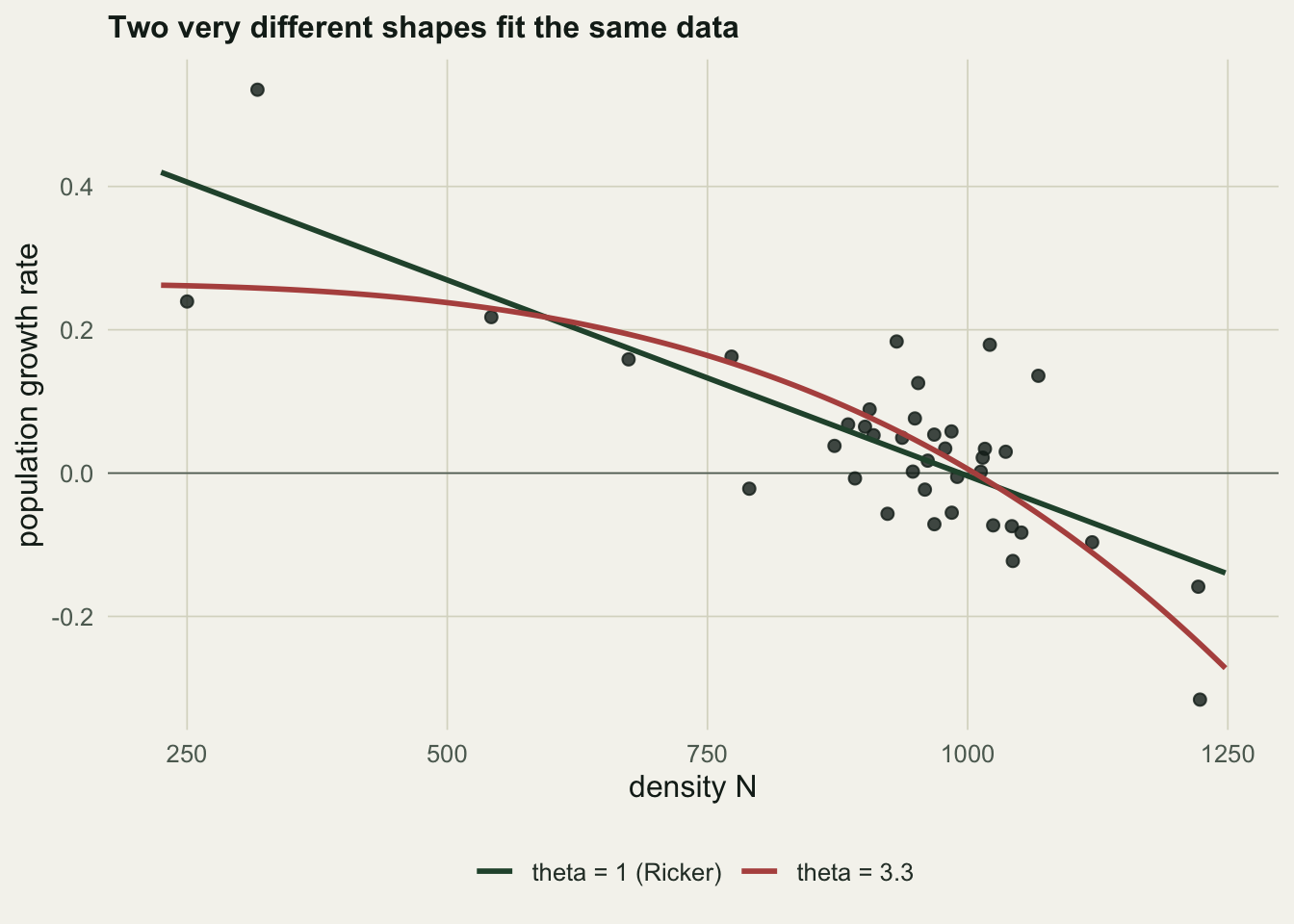

Figure 1: Population growth rate against density with two fitted theta-logistic curves. A Ricker shape and a sharply concave shape thread the same points, diverging only at low density where the data are sparse.

The Ricker fit sits only \(0.77\) log-likelihood units below the best fit, a deviance of about \(1.5\), well under the value of \(3.84\) that would mark a real difference. The sharply concave \(\theta = 3.3\) fit is close behind. Neither can be told apart from the maximum-likelihood shape on these data, and the two curves separate only in the low-density corner, where a settled population supplies few observations.

The likelihood ridge

Fixing the shape parameter at a grid of values and re-optimising the rest traces the profile likelihood for \(\theta\). It is nearly flat across a wide range, the ridge described by Polansky and colleagues.

tg <- seq(0.3, 6, length.out=80)
pl <- lapply(tg, function(x) fit_theta(N, x))
llp <- sapply(pl, function(z) z$ll); rp <- sapply(pl, function(z) z$r)
dev <- 2*(max(llp) - llp)
c(theta_lo=round(min(tg[dev<3.84]),1), theta_hi=round(max(tg[dev<3.84]),1),
  r_lo=round(min(rp[dev<3.84]),2), r_hi=round(max(rp[dev<3.84]),2))

theta_lo theta_hi     r_lo     r_hi 
    0.60     3.40     0.26     0.77 

d2 <- data.frame(theta=tg, dev=dev)
ggplot(d2, aes(theta, dev))+
  geom_hline(yintercept=3.84, colour=faint, linetype="22", linewidth=.4)+
  geom_line(colour=forest, linewidth=1)+
  geom_vline(xintercept=ff$theta, colour=aban, linewidth=.7)+
  geom_vline(xintercept=theta_true, colour=gold, linewidth=.7, linetype="22")+
  annotate("text", x=ff$theta, y=8, label=" MLE", hjust=0, colour=aban, size=3.3)+
  annotate("text", x=theta_true, y=6, label="truth ", hjust=1, colour="#8a7a1e", size=3.3)+
  annotate("text", x=5.4, y=3.84, label="95%", vjust=-0.5, colour=faint, size=3)+
  coord_cartesian(ylim=c(0,10))+
  labs(x="shape parameter theta (fixed)", y="profile deviance, relative to minimum",
       title="The shape parameter is barely identified")+
  theme_te()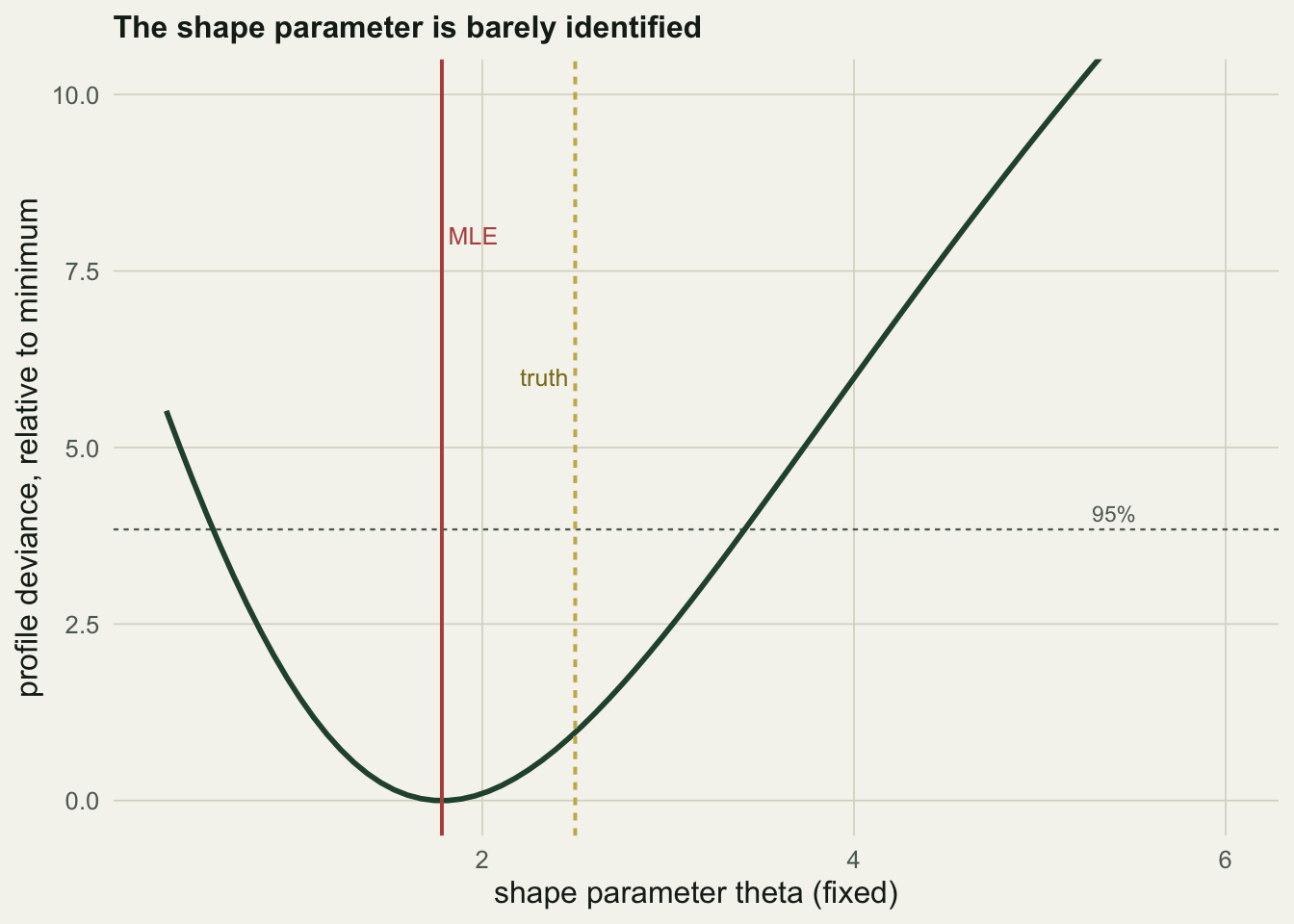

Figure 2: Profile deviance for the shape parameter. The curve stays below the 95 percent threshold across a wide band, so theta is only weakly identified, and the true value of 2.5 is well inside the interval.

Any shape between \(0.6\) and \(3.4\) falls within a likelihood interval of the best fit, so the data are consistent with a gentle Ricker curve, the true value of \(2.5\), and a sharp bend near the ceiling all at once. The reason the estimate is so loose is a trade-off with the growth rate: as \(\theta\) climbs along the ridge, the fitted \(r\) slides from \(0.77\) down to \(0.26\) to keep the predictions the same. Growth rate and shape are entangled, and one series cannot separate them.

What to do about it

The practical response is to stop trying to estimate the shape from a single series. Fixing \(\theta = 1\) and fitting the Ricker model is the common and defensible choice, and here it costs almost nothing in fit while removing an unidentified parameter; the extinction and density-dependence work in these posts uses that linear form for the same reason. Where the shape genuinely matters, the information has to come from elsewhere: a population pushed well below carrying capacity so the low-density curve is actually observed, several populations fitted together, or an informative prior in a Bayesian fit. The general lesson carries across this whole set of time-series methods. A model can be written down and fitted, and still contain parameters the data cannot resolve, so a profile likelihood is worth as much as the point estimate it surrounds. The same weak-identifiability caution applies to the density-dependence slope and to the split between process and observation error.

References

Polansky L, de Valpine P, Lloyd-Smith JO & Getz WM 2009 Ecology 90(8):2313-2320 (10.1890/08-1461.1)

Gilpin ME & Ayala FJ 1973 Proceedings of the National Academy of Sciences 70(12):3590-3593 (10.1073/pnas.70.12.3590)

Ricker WE 1954 Journal of the Fisheries Research Board of Canada 11(5):559-623 (10.1139/f54-039)

Related tutorials

• Detecting density dependence
• Extinction risk and population viability analysis
• The Gompertz state-space model
• Species-area relationships