library(ggplot2)

te_pal <- list(forest = "#275139", green = "#2f8f63", sage = "#93a87f",
               clay = "#b5534e", gold = "#cda23f", line = "#dad9ca",
               ink = "#16241d", paper = "#f5f4ee")

theme_te <- function() {
  theme_minimal(base_size = 12) +
    theme(panel.grid.minor = element_blank(),
          panel.grid.major = element_line(colour = "#e7e6dc"),
          plot.background = element_rect(fill = "#f5f4ee", colour = NA),
          panel.background = element_rect(fill = "#f5f4ee", colour = NA),
          plot.title = element_text(face = "bold", colour = te_pal$ink),
          axis.title = element_text(colour = "#2c3a31"))
}Surplus production models in R
R
fisheries
stock assessment
population dynamics
ecology tutorial
ggplot2
Fit a Schaefer biomass dynamics model to a catch series and an abundance index in R, and measure why a one-way trip leaves r, K and MSY badly identified.
Most fished stocks in the world have no age structure in their assessment, no survey of recruits and no tagging study. What they have is a catch series, because someone weighed the landings, and an index of abundance, because someone recorded catch per unit of effort or ran a trawl survey. A biomass dynamics model, also called a surplus production model, is the assessment you can still do with those two series. It treats the whole stock as one number, adds a production term, subtracts the catch, and asks which parameters make the observed index most likely.
The output is management currency: maximum sustainable yield, the biomass that produces it, and the fishing mortality that holds the stock there. Those numbers end up in harvest control rules and quota advice. This tutorial fits the model by hand in base R and then spends most of its length on the question that matters more than the fit: given a particular catch and index history, how well are they actually determined? We measure the likelihood profile over the growth rate and the carrying capacity, the correlation between them, and the spread of yield estimates that fit the data almost equally well.
If you have read the theta-logistic model in R you already know the logistic production curve and the shape of the trouble. There, an unharvested time series could not pin down the curvature parameter. Here the estimation problem differs in two ways that matter: the population is being removed from, so the catch series carries information about the scale of the stock, and abundance is never seen directly, only an index proportional to it by an unknown constant.
A production model and two fishing histories
The state equation is a bookkeeping identity plus one modelling assumption:
\[B_{t+1} = B_t + g(B_t) - C_t\]
where \(B_t\) is exploitable biomass at the start of year \(t\), \(C_t\) is the catch taken during it, and \(g\) is surplus production, the excess of growth and recruitment over natural mortality. Schaefer’s choice is the logistic, \(g(B) = rB(1 - B/K)\), which we later generalise. Biomass is never observed. Instead we see an index
\[I_t = qB_t \exp(\varepsilon_t), \qquad \varepsilon_t \sim N(0, \sigma^2)\]
with \(q\) the catchability coefficient that converts biomass into index units.
The two stocks below share every biological parameter and differ only in how they were fished. The first is fished up and then eased off: effort grows, the stock is pushed well below the level that produces most yield, managers cut effort, and the stock recovers. The second is a one-way trip, the pattern that dominates real assessment data, with effort growing and biomass falling every year.
set.seed(20260818)

production <- function(bio, rr, kk, shape) (rr / shape) * bio * (1 - (bio / kk)^shape)

sim_stock <- function(rr, kk, qq, fpath, sig_obs, sig_proc = 0) {
  nyr <- length(fpath)
  bio <- numeric(nyr + 1)
  catch <- numeric(nyr)
  bio[1] <- kk
  for (i in seq_len(nyr)) {
    catch[i] <- fpath[i] * bio[i]
    nxt <- bio[i] + production(bio[i], rr, kk, 1) - catch[i]
    if (sig_proc > 0) nxt <- nxt * exp(rnorm(1, -sig_proc^2 / 2, sig_proc))
    bio[i + 1] <- max(nxt, 1e-6)
  }
  cpue <- qq * bio[seq_len(nyr)] * exp(rnorm(nyr, -sig_obs^2 / 2, sig_obs))
  data.frame(year = seq_len(nyr), biomass = bio[seq_len(nyr)],
             catch = catch, cpue = cpue)
}

r_true <- 0.32; k_true <- 1200; q_true <- 3.5e-4; sig_obs <- 0.12; nyr <- 40

f_con <- c(seq(0.02, 0.30, length.out = 14), rep(0.30, 6),
           seq(0.30, 0.05, length.out = 4), rep(0.05, 6), rep(0.15, 10))
f_one <- seq(0.015, 0.34, length.out = nyr)

d_con <- sim_stock(r_true, k_true, q_true, f_con, sig_obs)
d_one <- sim_stock(r_true, k_true, q_true, f_one, sig_obs)

c(years = nyr, index_cv = sig_obs)
years index_cv
40.00 0.12 round(c(true_r = r_true, true_K = k_true, true_q = q_true,
true_MSY = r_true * k_true / 4, true_Bmsy = k_true / 2,
true_Fmsy = r_true / 2), 5) true_r true_K true_q true_MSY true_Bmsy true_Fmsy
3.2e-01 1.2e+03 3.5e-04 9.6e+01 6.0e+02 1.6e-01 round(c(contrast_lowest_BK = min(d_con$biomass) / k_true,
contrast_final_BK = d_con$biomass[nyr] / k_true,
oneway_final_BK = d_one$biomass[nyr] / k_true,
oneway_declines_every_year = as.numeric(all(diff(d_one$biomass) < 0))), 3) contrast_lowest_BK contrast_final_BK
0.215 0.545
oneway_final_BK oneway_declines_every_year
0.188 1.000 The contrast stock is driven down to 0.215 of carrying capacity and recovers to 0.545 of it. The one-way stock ends at 0.188 of carrying capacity, having fallen in every one of its 40 years. Both are observed through an index with a coefficient of variation of 0.12, which is optimistic for a real catch rate series.
long <- rbind(
  data.frame(d_con, stock = "Contrast: fished down, then rebuilt"),
  data.frame(d_one, stock = "One-way trip: effort only grows"))
long$biomass <- long$biomass / k_true
panels <- rbind(
  data.frame(long[, c("year", "stock")], value = long$biomass,
             panel = "Biomass / K"),
  data.frame(long[, c("year", "stock")], value = long$catch,
             panel = "Catch"),
  data.frame(long[, c("year", "stock")], value = long$cpue,
             panel = "Index"))
panels$panel <- factor(panels$panel, levels = c("Biomass / K", "Catch", "Index"))

ggplot(panels, aes(year, value)) +
  geom_line(colour = te_pal$forest, linewidth = 0.7) +
  geom_point(colour = te_pal$green, size = 0.9) +
  facet_grid(panel ~ stock, scales = "free_y") +
  labs(x = "Year", y = NULL, title = "Same biology, two management histories") +
  theme_te() +
  theme(strip.text = element_text(colour = te_pal$ink, face = "bold"))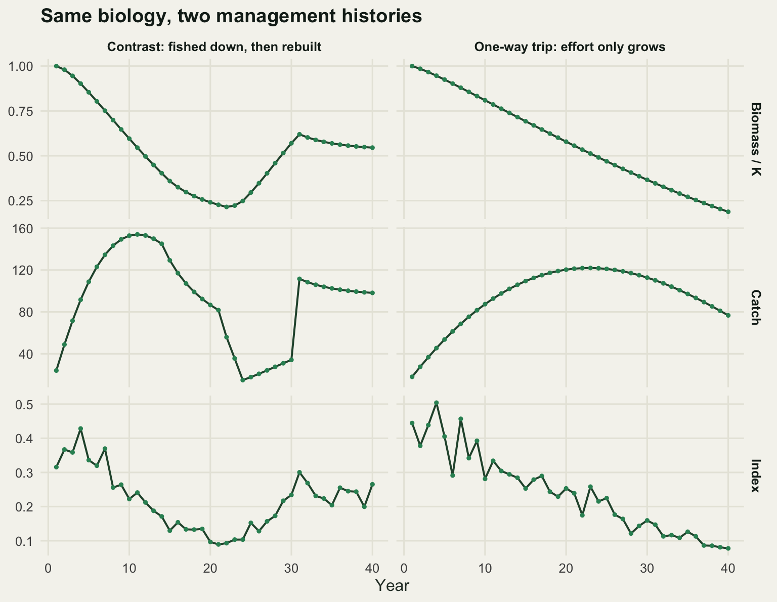
Fitting the model and reading off the reference points
The likelihood is written for the index, conditional on the catch. Given a candidate pair \((r, K)\), the biomass path is not random: start at \(B_1 = K\) and step the state equation forward, subtracting the observed catch each year. That gives a predicted biomass for every year, and the only free parameters left are the catchability and the observation standard deviation. Both drop out analytically. For a lognormal index the maximum likelihood catchability is the geometric mean ratio of index to biomass, so \(\log \hat{q}\) is the mean of \(\log I_t - \log B_t\); the residual variance is then the mean squared deviation about that mean. Substituting both back leaves a function of two parameters only.
One constraint has to go in by hand. A candidate pair can describe a stock too small to have produced the catch that was actually landed, and then the projected biomass passes through zero. Those pairs are rejected rather than kept on a floored path, because a floored path is a trajectory that never happened, and it plants sharp spurious minima in the likelihood exactly where the stock sits on the edge of collapse. The rule below drops any pair whose path falls under one per cent of its own carrying capacity; the floor that still appears in the recursion only keeps the stored biomass matrix positive, and any pair that touches it has already been flagged for rejection.
The function is written to take vectors of \(r\) and \(K\) at once, because we will later evaluate it on a grid of tens of thousands of parameter pairs. The recursion runs over years, not over parameter values, so the whole grid costs about as much as one loop.
project_biomass <- function(rv, kv, catch, shape = 1) {
  nyr <- length(catch)
  bio <- matrix(0, nrow = length(rv), ncol = nyr)
  bio[, 1] <- kv
  ok <- rep(TRUE, length(rv))
  for (i in seq_len(nyr - 1)) {
    nxt <- bio[, i] + production(bio[, i], rv, kv, shape) - catch[i]
    ok <- ok & is.finite(nxt) & nxt > 0.01 * kv
    bio[, i + 1] <- pmax(nxt, 0.01 * kv)
  }
  list(bio = bio, ok = ok)
}

spm_nll <- function(rv, kv, catch, cpue, shape = 1) {
  path <- project_biomass(rv, kv, catch, shape)
  lres <- matrix(log(cpue), nrow = length(rv), ncol = length(cpue),
                 byrow = TRUE) - log(path$bio)
  s2 <- rowMeans(lres^2) - rowMeans(lres)^2
  s2[!is.finite(s2) | s2 <= 0] <- 1e-12
  out <- 0.5 * length(cpue) * (log(2 * pi * s2) + 1)
  out[!path$ok] <- 1e6
  out
}

fit_spm <- function(dat, shape = 1, init = c(log(0.3), log(1000))) {
  obj <- function(par) spm_nll(exp(par[1]), exp(par[2]), dat$catch, dat$cpue, shape)
  opt <- optim(init, obj, control = list(reltol = 1e-13, maxit = 2000))
  opt <- optim(opt$par, obj, control = list(reltol = 1e-13, maxit = 2000))
  rr <- exp(opt$par[1]); kk <- exp(opt$par[2])
  bio <- as.vector(project_biomass(rr, kk, dat$catch, shape)$bio)
  list(r = rr, K = kk, q = exp(mean(log(dat$cpue) - log(bio))),
       shape = shape, nll = opt$value, bio = bio,
       bmsy = kk * (1 + shape)^(-1 / shape),
       msy = rr * kk * (1 + shape)^(-(1 + shape) / shape),
       fmsy = rr / (1 + shape))
}

fit_con <- fit_spm(d_con)
round(c(r = fit_con$r, K = fit_con$K, q = fit_con$q,
        MSY = fit_con$msy, Bmsy = fit_con$bmsy, Fmsy = fit_con$fmsy), 5)
r K q MSY Bmsy Fmsy
0.30539 1240.81511 0.00033 94.73342 620.40756 0.15270 round(c(r_pct_error = 100 * (fit_con$r / r_true - 1),
K_pct_error = 100 * (fit_con$K / k_true - 1),
q_pct_error = 100 * (fit_con$q / q_true - 1),
MSY_pct_error = 100 * (fit_con$msy / (r_true * k_true / 4) - 1)), 2) r_pct_error K_pct_error q_pct_error MSY_pct_error
-4.57 3.40 -6.09 -1.32 On the contrast stock the fit recovers everything: the growth rate is 4.57 per cent low, the carrying capacity 3.4 per cent high, the catchability 6.09 per cent low, and the errors partly cancel in the yield, which is 1.32 per cent low. The estimated maximum sustainable yield of 94.73 sits against a true value of 96.
The Schaefer reference points have closed forms. Production is a downward parabola in biomass, so it peaks exactly halfway to carrying capacity: \(B_{MSY} = K/2\), \(MSY = rK/4\), and the fishing mortality holding the stock at that peak is \(F_{MSY} = MSY / B_{MSY} = r/2\). Confirm that on the fitted curve rather than trusting the algebra, because the same code has to work later for a production curve with no such tidy solution.
bgrid <- seq(1, fit_con$K, length.out = 200001)
pgrid <- production(bgrid, fit_con$r, fit_con$K, 1)
round(c(numeric_Bmsy = bgrid[which.max(pgrid)],
        closed_form_K_over_2 = fit_con$K / 2,
        numeric_MSY = max(pgrid),
        closed_form_rK_over_4 = fit_con$r * fit_con$K / 4,
        numeric_Fmsy = max(pgrid) / bgrid[which.max(pgrid)],
        closed_form_r_over_2 = fit_con$r / 2), 4)
numeric_Bmsy closed_form_K_over_2 numeric_MSY
620.4054 620.4076 94.7334
closed_form_rK_over_4 numeric_Fmsy closed_form_r_over_2
94.7334 0.1527 0.1527 Searching the fitted production curve numerically gives a peak at a biomass of 620.4054 against the closed form 620.4076, a yield of 94.7334 matching rK/4 to four decimal places, and a fishing mortality of 0.1527 matching r/2. The algebra is right, and it will be the algebra that misleads us later, not the arithmetic.
The one-way trip
Now fit the same model to the declining stock. The point estimates look reassuring.
fit_one <- fit_spm(d_one)
round(c(r = fit_one$r, K = fit_one$K, q = fit_one$q,
        MSY = fit_one$msy, Bmsy = fit_one$bmsy, Fmsy = fit_one$fmsy), 5)
r K q MSY Bmsy Fmsy
0.29754 1267.28943 0.00032 94.26795 633.64472 0.14877 A growth rate of 0.29754 and a carrying capacity of 1267.28 against a truth of 0.32 and 1200, with a yield estimate of 94.27 against 96. If you stopped here you would conclude that a one-way trip is fine. On this run the point estimate is not the problem. The problem is everything else that fits nearly as well, and to see it you have to look at the likelihood surface rather than at its maximum.
r_cap <- 1
rgrid <- exp(seq(log(0.02), log(r_cap), length.out = 200))
kgrid <- exp(seq(log(250), log(30000), length.out = 200))
c(search_box_r = range(rgrid), search_box_K = range(kgrid))
search_box_r1 search_box_r2 search_box_K1 search_box_K2
2.0e-02 1.0e+00 2.5e+02 3.0e+04 surf <- expand.grid(r = rgrid, K = kgrid)
surf$dev_con <- spm_nll(surf$r, surf$K, d_con$catch, d_con$cpue)
surf$dev_con <- 2 * (surf$dev_con - min(surf$dev_con))
surf$dev_one <- spm_nll(surf$r, surf$K, d_one$catch, d_one$cpue)
surf$dev_one <- 2 * (surf$dev_one - min(surf$dev_one))
in_con <- surf[surf$dev_con <= 4, ]
in_one <- surf[surf$dev_one <= 4, ]
round(c(grid_points = nrow(surf),
inside_contrast = nrow(in_con), inside_oneway = nrow(in_one),
cor_logr_logK_contrast = cor(log(in_con$r), log(in_con$K)),
cor_logr_logK_oneway = cor(log(in_one$r), log(in_one$K))), 4) grid_points inside_contrast inside_oneway
40000.0000 4.0000 78.0000
cor_logr_logK_contrast cor_logr_logK_oneway
-1.0000 -0.9872 The searched box is generous but not unlimited: growth rates from 0.02 to 1 and carrying capacities from 250 to 30000 tonnes. A growth rate above 1 is not a fish stock, and it also drives the discrete recursion towards the oscillating part of its behaviour, where the likelihood stops meaning anything.
Out of 40000 grid points, 4 lie within two log-likelihood units of the best fit for the contrast stock and 78 do for the one-way trip. Inside the one-way set the correlation between log r and log K is -0.9872. Both surfaces are the same ridge: the parameters trade off almost perfectly against each other, so a lower growth rate is absorbed by a higher carrying capacity, though not one for one. The carrying capacity has to move proportionally less than the growth rate does. The difference is how far along that ridge the data let you slide.
ridge <- rbind(
  data.frame(surf[, c("r", "K")], dev = surf$dev_con,
             stock = "Contrast: fished down, then rebuilt"),
  data.frame(surf[, c("r", "K")], dev = surf$dev_one,
             stock = "One-way trip: effort only grows"))
best_k <- function(dv) {
  mat <- matrix(dv, nrow = length(rgrid), ncol = length(kgrid))
  kgrid[apply(mat, 1, which.min)]
}
trace_ridge <- rbind(
  data.frame(r = rgrid, K = best_k(surf$dev_con),
             stock = "Contrast: fished down, then rebuilt"),
  data.frame(r = rgrid, K = best_k(surf$dev_one),
             stock = "One-way trip: effort only grows"))
marks <- data.frame(
  r = c(r_true, fit_con$r, r_true, fit_one$r),
  K = c(k_true, fit_con$K, k_true, fit_one$K),
  kind = rep(c("truth", "fitted"), 2),
  stock = rep(c("Contrast: fished down, then rebuilt",
                "One-way trip: effort only grows"), each = 2))

ggplot(ridge, aes(r, K, z = dev)) +
  geom_contour_filled(breaks = c(0, 4, 10, 25, 60, Inf)) +
  geom_line(data = trace_ridge, aes(r, K), inherit.aes = FALSE,
            colour = te_pal$gold, linewidth = 0.5, linetype = "22") +
  geom_point(data = marks, aes(r, K, shape = kind), inherit.aes = FALSE,
             colour = te_pal$clay, size = 3, stroke = 1.2) +
  scale_fill_manual(values = c("#275139", "#3f9970", "#93a87f",
                               "#c4cfb6", "#e6e4d6"), name = "Deviance") +
  scale_shape_manual(values = c(truth = 1, fitted = 4), name = NULL) +
  scale_x_log10() + scale_y_log10() +
  coord_cartesian(xlim = c(0.02, 1), ylim = c(350, 20000)) +
  facet_wrap(~stock) +
  labs(x = "Growth rate r", y = "Carrying capacity K", title = "One likelihood ridge, two lengths") +
  theme_te() +
  theme(strip.text = element_text(colour = te_pal$ink, face = "bold"))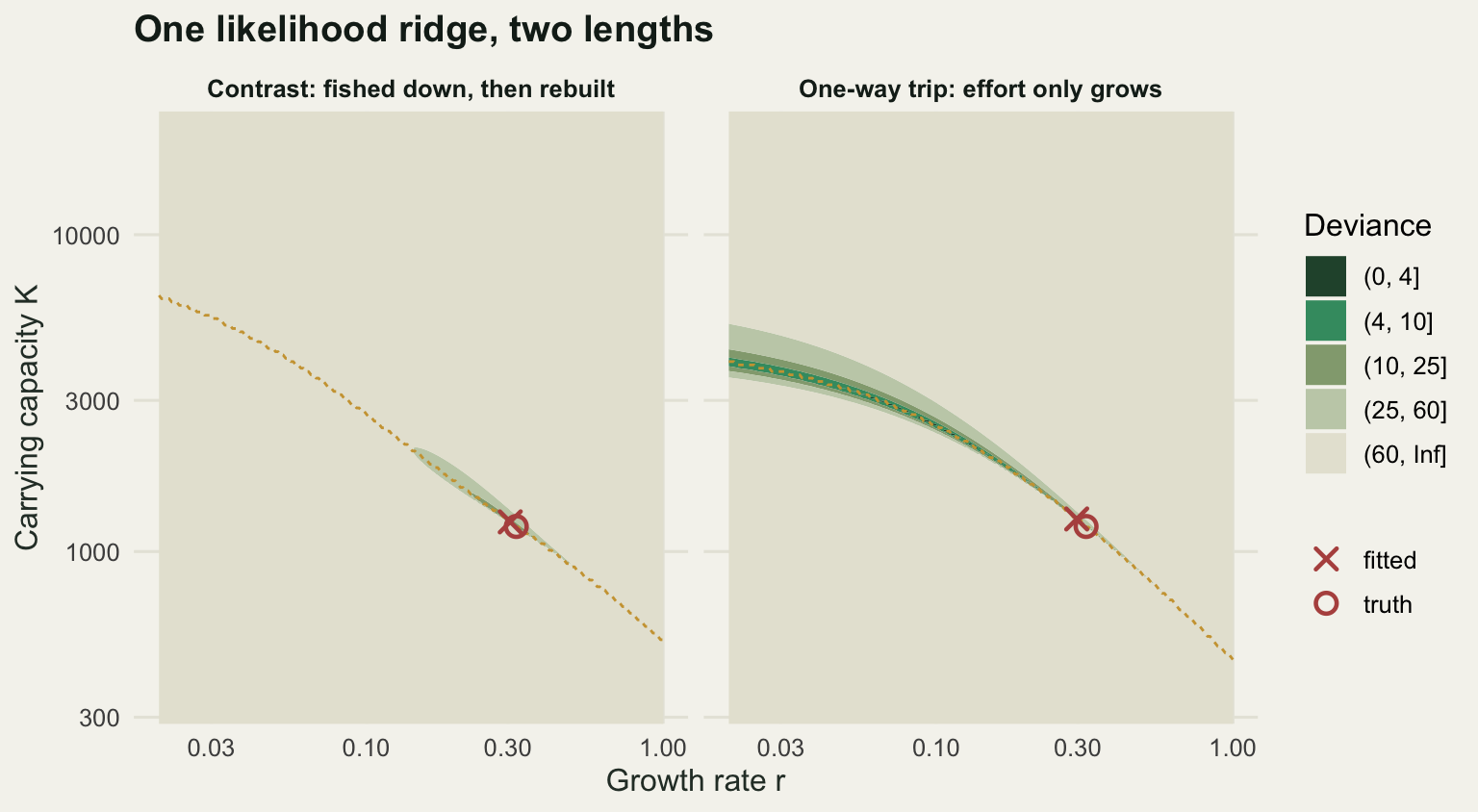
The picture explains what the catch and index series can and cannot say. The index tells you the relative shape of the biomass trajectory. The catch tells you, in tonnes, how much had to be removed to produce that shape. Together they pin down the early rate of decline, which is close to a product of the two parameters, and they pin it down well. What separates r from K is information about how fast the stock replaces itself at low biomass, and a stock that has only been going down has never been observed replacing itself.
What breaks the ridge
The fix is more informative data, not a better optimiser. To show that with the least possible confounding, take the contrast series and truncate it at the end of the decline, before the recovery. The stock, the biology and the estimator are all identical; only the years differ.
d_trunc <- d_con[seq_len(22), ]
c(truncated_years = nrow(d_trunc))
truncated_years
22 # profile: minimise over the nuisance parameter on a grid, then refine locally
prof_min <- function(dat, xv, ygrid, build, shape = 1) {
cost <- function(xx, yv) {
pars <- build(xx, yv)
spm_nll(pars$r, pars$K, dat$catch, dat$cpue, shape)
}
dv <- sapply(xv, function(xx) {
vals <- cost(xx, ygrid)
j <- which.min(vals)
lo <- ygrid[max(j - 1, 1)]
hi <- ygrid[min(j + 1, length(ygrid))]
if (lo >= hi) return(vals[j])
min(vals[j],
optimize(function(ly) cost(xx, exp(ly)), c(log(lo), log(hi)), tol = 1e-9)$objective)
})
data.frame(value = xv, dev = 2 * (dv - min(dv)))
}
build_r <- function(xx, yv) list(r = rep(xx, length(yv)), K = yv)
build_k <- function(xx, yv) list(r = yv, K = rep(xx, length(yv)))
build_msy <- function(xx, yv) {
rr <- xx / (0.25 * yv)
rr[rr > r_cap] <- 1e3 # outside the search box
list(r = rr, K = yv)
}
mgrid <- exp(seq(log(5), log(300), length.out = 200))
series <- list(contrast = d_con, truncated = d_trunc, oneway = d_one)
mp <- lapply(series, function(dat) prof_min(dat, rgrid, kgrid, build_r))
kp <- lapply(series, function(dat) prof_min(dat, kgrid, rgrid, build_k))
mm <- lapply(series, function(dat) prof_min(dat, mgrid, kgrid, build_msy))
# where the profile crosses two log-likelihood units, by interpolation
span <- function(pf) {
ok <- which(pf$dev <= 4)
cross <- function(i, j) exp(approx(pf$dev[c(i, j)], log(pf$value[c(i, j)]), 4)$y)
lo <- if (min(ok) == 1) pf$value[1] else cross(min(ok) - 1, min(ok))
hi <- if (max(ok) == nrow(pf)) pf$value[nrow(pf)] else cross(max(ok) + 1, max(ok))
c(lo = lo, hi = hi, fold = hi / lo,
at_edge = as.numeric(min(ok) == 1 || max(ok) == nrow(pf)))
}
prof_tab <- data.frame(r = t(sapply(mp, span)), K = t(sapply(kp, span)),
MSY = t(sapply(mm, span)))
print(round(prof_tab, 3)) r.lo r.hi r.fold r.at_edge K.lo K.hi K.fold K.at_edge
contrast 0.275 0.339 1.233 0 1158.061 1331.020 1.149 0
truncated 0.020 0.304 15.218 1 1246.185 2941.995 2.361 0
oneway 0.046 1.000 21.933 1 456.188 3343.464 7.329 0
MSY.lo MSY.hi MSY.fold MSY.at_edge
contrast 91.437 98.051 1.072 0
truncated 5.000 94.858 18.972 1
oneway 38.083 111.805 2.936 0fit_tr <- fit_spm(d_trunc)
round(c(truncated_MSY_point = fit_tr$msy, truncated_r_point = fit_tr$r,
truncated_K_point = fit_tr$K,
truncated_MSY_pct_error = 100 * (fit_tr$msy / (r_true * k_true / 4) - 1)), 3) truncated_MSY_point truncated_r_point truncated_K_point
55.225 0.107 2062.853
truncated_MSY_pct_error
-42.474 grab_prof <- function(nm) rbind(
data.frame(mp[[nm]], parameter = "Growth rate r", series = nm),
data.frame(kp[[nm]], parameter = "Carrying capacity K", series = nm),
data.frame(mm[[nm]], parameter = "MSY", series = nm))
prof_long <- do.call(rbind, lapply(names(series), grab_prof))
prof_long$parameter <- factor(prof_long$parameter, levels = c(
"Growth rate r", "Carrying capacity K", "MSY"))
prof_long$series <- factor(prof_long$series, levels = c(
"contrast", "truncated", "oneway"), labels = c(
"contrast (40 y)", "truncated (22 y)", "one-way trip (40 y)"))
ggplot(prof_long, aes(value, dev, colour = series)) +
geom_hline(yintercept = 4, colour = te_pal$line, linewidth = 0.8) +
geom_line(linewidth = 0.8) +
facet_wrap(~parameter, scales = "free_x") +
scale_x_log10() +
scale_colour_manual(values = c(te_pal$forest, te_pal$gold, te_pal$clay),
name = NULL) +
coord_cartesian(ylim = c(0, 14)) +
labs(x = "Parameter value", y = "Deviance from best fit", title = "What a rebuild adds to the likelihood") +
theme_te() +
theme(legend.position = "top",
strip.text = element_text(colour = te_pal$ink, face = "bold"))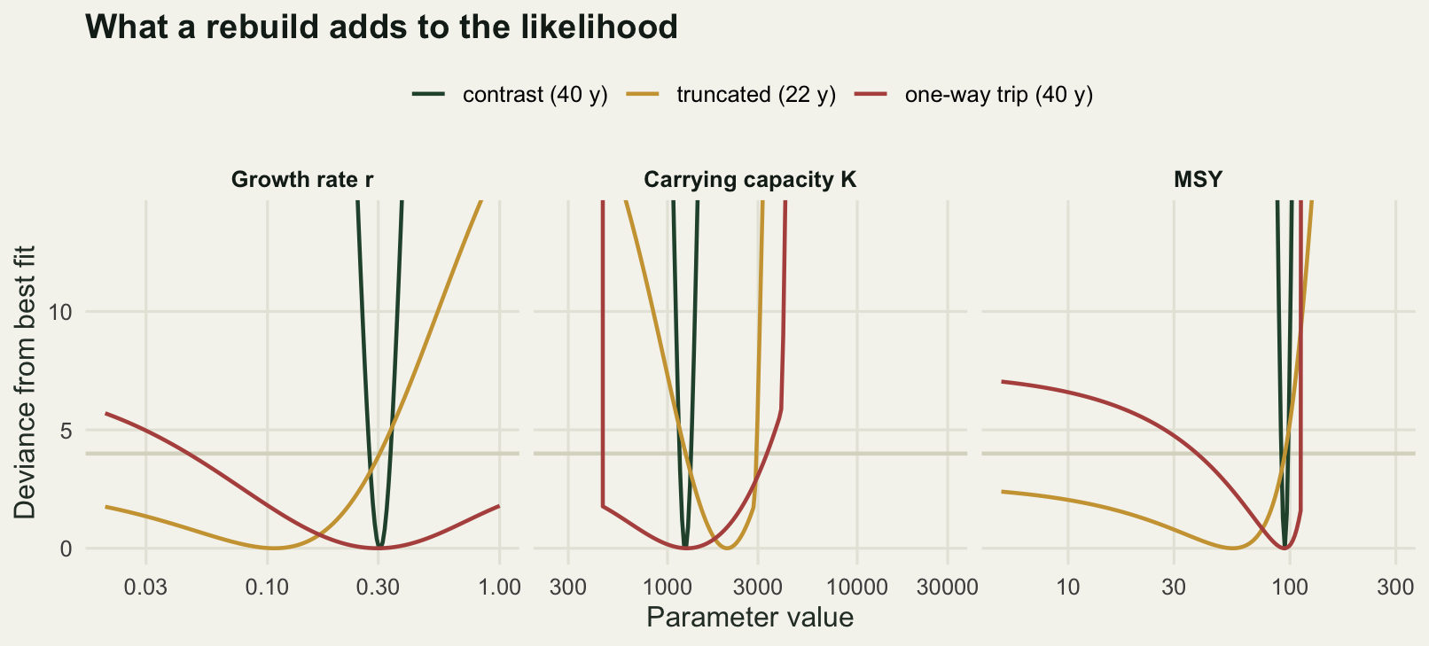
Read the table by the fold columns, the ratio of the top of the two-unit interval to its bottom, and by the at_edge flag, which is 1 when the interval runs out of the box we searched. With the full contrast series the growth rate is determined to within a factor of 1.233, the carrying capacity to 1.149 and the yield to 1.072. On the one-way trip the growth rate interval reaches the top of the box, so its 21.933 is a lower bound on the fold range rather than a measurement, and the carrying capacity spans 7.329-fold only because we refused to consider growth rates above 1. Yield is the one quantity the one-way trip bounds on both sides on this run: anything between 38.083 and 111.805 tonnes fits within two log-likelihood units, a 2.936-fold range, so an assessment could defend a quota near the top of that range or near the bottom without the data objecting.
The truncated series is in the same trouble as the one-way trip, which surprised me until I looked at the figure. Its growth rate profile runs down to 0.02 and its yield profile down to 5, both of which are the bottom of the searched box rather than anything the data said. The profile is flat: a stock with almost no production at all, being mined down by the catch, fits those 22 years as well as anything else does. The point estimate is not flat, and that is the trap. It comes back with a growth rate of 0.107, a carrying capacity of 2062.853 and a yield of 55.225 tonnes, which is 42.474 per cent below the truth, reported to three decimal places by an optimiser that converged cleanly.
Eighteen more years, containing a period of low exploitation and a visible rebuild, turn an unbounded yield estimate into one pinned to a 1.072-fold range. No amount of care with starting values, priors or optimiser settings would have done that.
Pella-Tomlinson and the shape of production
Schaefer’s parabola puts peak production exactly at half of carrying capacity. That is a strong claim about a fish stock and nothing in the data forced it. The Pella-Tomlinson generalisation adds a shape parameter,
\[g(B) = \frac{r}{p} B \left( 1 - (B/K)^p \right),\]
which recovers Schaefer at \(p = 1\), moves the production peak down towards \(B_{MSY}/K = 1/e\) as \(p\) approaches zero, and pushes it up above half of carrying capacity for \(p > 1\). The reference points keep closed forms: \(B_{MSY}/K = (1 + p)^{-1/p}\), \(F_{MSY} = r/(1 + p)\) and \(MSY = rK(1 + p)^{-(1+p)/p}\).
We profile the shape parameter on the contrast series, the best behaved of our three, refitting r and K at each value.
fit_shape <- function(dat, shape) {
  ff <- fit_spm(dat, shape, init = c(log(0.3), log(1200)))
  data.frame(shape = shape, r = ff$r, K = ff$K, nll = ff$nll, bmsy = ff$bmsy,
             bratio = ff$bmsy / ff$K, msy = ff$msy, fmsy = ff$fmsy)
}

shape_grid <- exp(seq(log(0.1), log(8), length.out = 45))
shape_tab <- do.call(rbind, lapply(shape_grid, function(s) fit_shape(d_con, s)))
shape_tab$dev <- 2 * (shape_tab$nll - min(shape_tab$nll))
ok_shape <- shape_tab$shape[shape_tab$dev <= 4]

round(c(best_shape = shape_tab$shape[which.min(shape_tab$dev)],
        shape_lo = min(ok_shape), shape_hi = max(ok_shape),
        shape_fold = max(ok_shape) / min(ok_shape),
        deviance_at_shape_one = shape_tab$dev[which.min(abs(shape_tab$shape - 1))]), 2)
best_shape shape_lo shape_hi
1.80 0.99 2.67
shape_fold deviance_at_shape_one
2.71 3.92 shape_long <- rbind(
data.frame(shape = shape_tab$shape, value = shape_tab$dev,
panel = "Profile deviance"),
data.frame(shape = shape_tab$shape, value = shape_tab$bratio,
panel = "Implied Bmsy / K"))
panel_order <- c("Profile deviance", "Implied Bmsy / K")
shape_long$panel <- factor(shape_long$panel, levels = panel_order)
inside <- data.frame(lo = min(ok_shape), hi = max(ok_shape))
cutline <- data.frame(yv = 4,
panel = factor("Profile deviance", levels = panel_order))
ggplot(shape_long, aes(shape, value)) +
geom_rect(data = inside, aes(xmin = lo, xmax = hi, ymin = -Inf, ymax = Inf),
inherit.aes = FALSE, fill = te_pal$sage, alpha = 0.25) +
geom_hline(data = cutline, aes(yintercept = yv),
colour = te_pal$clay, linewidth = 0.5, linetype = "22") +
geom_line(colour = te_pal$forest, linewidth = 0.8) +
facet_wrap(~panel, ncol = 1, scales = "free_y") +
scale_x_log10() +
labs(x = "Shape parameter p", y = NULL, title = "A shape the data cannot choose") +
theme_te() +
theme(strip.text = element_text(colour = te_pal$ink, face = "bold"))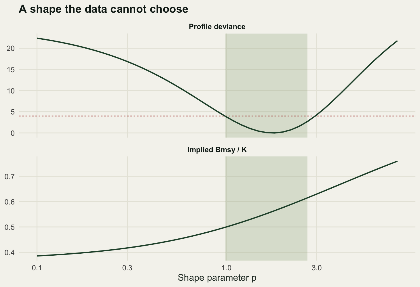
The profile has its minimum at a shape of 1.8, when the truth is 1, and any shape between 0.99 and 2.67 lies within two log-likelihood units. That is a 2.71-fold range on a parameter whose whole job is to say where the stock is most productive. On this run Schaefer itself sits at a deviance of 3.92, just inside the interval: the data do not reject it and do not prefer it either. This is the same failure as the curvature parameter in the theta-logistic tutorial, arriving by a different route.
The consequence is not academic, because the shape is usually fixed by the analyst rather than estimated. Compare a fixed Schaefer against a fixed shape of 3, which skews production towards higher biomass, on exactly the same data.
s1 <- fit_shape(d_con, 1)
s3 <- fit_shape(d_con, 3)
print(round(rbind(schaefer = unlist(s1), skewed = unlist(s3)), 4))
shape r K nll bmsy bratio msy fmsy
schaefer 1 0.3054 1240.815 -31.5892 620.4075 0.50 94.7334 0.1527
skewed 3 0.5913 1118.232 -31.3471 704.4418 0.63 104.1407 0.1478bmsy_pct_shift <- 100 * (s3$bmsy / s1$bmsy - 1)
round(c(MSY_pct_shift = 100 * (s3$msy / s1$msy - 1),
Bmsy_pct_shift = bmsy_pct_shift,
Fmsy_pct_shift = 100 * (s3$fmsy / s1$fmsy - 1),
deviance_gap = 2 * (s3$nll - s1$nll)), 2) MSY_pct_shift Bmsy_pct_shift Fmsy_pct_shift deviance_gap
9.93 13.55 -3.18 0.48 The two fits are separated by a deviance of 0.48. Yet the biomass target moves from 620.4075 to 704.4418 tonnes, 13.55 per cent higher, and the yield from 94.7334 to 104.1407, 9.93 per cent higher. The fishing mortality target barely moves at all, from 0.1527 to 0.1478. That asymmetry is the practical lesson: the shape assumption is close to invisible in the exploitation rate advice and highly visible in the biomass target, which is the number a rebuilding plan is written against. Choosing p is a management decision that arrives dressed as a modelling convenience.
Where the error lives
The model above puts all of its error in the index and none in the dynamics: biomass follows the state equation exactly and the index wanders around it. The opposite assumption is just as easy to code. Treat the index as an exact scaled measurement, so that \(B_t = I_t / q\), and put the noise in the production process instead. The residuals become the log ratios of observed to predicted biomass one step ahead, and catchability has to be estimated rather than concentrated out.
set.seed(4021)
sig_proc <- 0.15
d_proc <- sim_stock(r_true, k_true, q_true, f_con, 0.03, sig_proc)

nll_proc <- function(par, dat) {
  rr <- exp(par[1]); kk <- exp(par[2]); qq <- exp(par[3])
  bio <- dat$cpue / qq
  nn <- length(bio)
  pred <- bio[-nn] + production(bio[-nn], rr, kk, 1) - dat$catch[-nn]
  if (any(!is.finite(pred)) || any(pred <= 0)) return(1e8)
  wres <- log(bio[-1]) - log(pred)
  s2 <- mean(wres^2)
  if (!is.finite(s2) || s2 <= 0) return(1e8)
  0.5 * length(wres) * (log(2 * pi * s2) + 1)
}

fit_proc <- function(dat) {
  init <- c(log(0.3), log(1200), log(median(dat$cpue) / 600))
  opt <- optim(init, nll_proc, dat = dat, control = list(reltol = 1e-13, maxit = 4000))
  opt <- optim(opt$par, nll_proc, dat = dat, control = list(reltol = 1e-13, maxit = 4000))
  rr <- exp(opt$par[1]); kk <- exp(opt$par[2])
  list(r = rr, K = kk, q = exp(opt$par[3]), msy = rr * kk / 4, bmsy = kk / 2)
}

grab <- function(f) c(r = f$r, K = f$K, q = f$q, MSY = f$msy)
print(round(rbind(
  truth              = c(r = r_true, K = k_true, q = q_true, MSY = r_true * k_true / 4),
  index_error_obsfit = grab(fit_spm(d_con)),
  index_error_procfit = grab(fit_proc(d_con)),
  process_error_obsfit = grab(fit_spm(d_proc)),
  process_error_procfit = grab(fit_proc(d_proc))), 5))
r K q MSY
truth 0.32000 1200.000 0.00035 96.00000
index_error_obsfit 0.30539 1240.815 0.00033 94.73342
index_error_procfit 0.36796 1120.752 0.00034 103.09801
process_error_obsfit 0.34226 1247.141 0.00038 106.71303
process_error_procfit 0.35276 1241.323 0.00033 109.47269On the index-error data the observation-error fit gives a yield of 94.73342 and the process-error fit gives 103.09801. On the process-error data they give 106.71303 and 109.47269. A single realisation cannot separate bias from luck, so repeat the whole exercise.
set.seed(88)
nrep <- 60
mc <- do.call(rbind, lapply(seq_len(nrep), function(i) {
  da <- sim_stock(r_true, k_true, q_true, f_con, sig_obs, 0)
  db <- sim_stock(r_true, k_true, q_true, f_con, 0.03, sig_proc)
  data.frame(rep = i,
             truth = rep(c("index error", "process error"), each = 2),
             assumption = rep(c("observation", "process"), 2),
             msy = c(fit_spm(da)$msy, fit_proc(da)$msy,
                     fit_spm(db)$msy, fit_proc(db)$msy))
}))
mc$ratio <- mc$msy / (r_true * k_true / 4)

c(replicates = nrep)
replicates
60 print(round(tapply(mc$ratio, list(mc$truth, mc$assumption), median), 3)) observation process
index error 1.009 1.084
process error 0.927 0.959print(round(tapply(mc$ratio, list(mc$truth, mc$assumption), mad), 3)) observation process
index error 0.015 0.04
process error 0.133 0.14Over 60 replicates, the median ratio of estimated to true yield is 1.009 when the observation error assumption is correct and the observation error estimator is used, and 1.084 when the same data are fitted assuming the noise is in the dynamics. Reverse the truth and the observation error estimator returns 0.927 while the correctly specified process error estimator returns 0.959. Neither wrong assumption is a catastrophe here, but the scatter is not symmetric: the median absolute deviation of the ratio is 0.015 for the matched observation error case and 0.04 for the mismatched one, so the mistake widens the spread as well as shifting the centre.
The standard surplus production model, the one implemented in most assessment software, assumes observation error only. On this evidence that is the safer default: very precise when it is right, about 7 per cent low on the yield when it is wrong. State space versions carrying both error types are now common practice and they are the honest answer, but splitting the two variances needs either a strong prior or more contrast than a one-way trip provides.
What the model cannot tell you
A biomass dynamics model has no age structure. Every tonne is the same as every other tonne, so a stock that has lost its large old fish while holding its total weight looks healthy, and years of recruitment failure stay invisible until the biomass they should have become fails to appear. The model absorbs that as a lower growth rate, which is the wrong diagnosis if the cause was a temporary change in the environment.
It also assumes the index is proportional to biomass with a constant catchability. Fleets learn, gear changes, and boats concentrate on the remaining aggregations as a stock declines, all of which make catch rates fall more slowly than abundance. Under that kind of drift the index looks like a stock that is holding up, and the model reads it as high productivity. Standardising the index is a separate piece of work and the third post of this cluster does it.
The deepest limit is the one the profiles were pointing at all along. Maximum sustainable yield is a property of a fitted model, not of a fish stock. It is the peak of a curve that we chose the shape of, fitted to data that could not tell us the shape, using a parameterisation in which two of the parameters are nearly unidentifiable from each other. It is still useful, and the fisheries that ignore it do worse. But a yield estimate deserves the profile that produced it printed next to it, and the two-unit interval on the one-way trip spanned a factor of 2.936.
Where to go next
The obvious repair for a model with no age structure is to put recruitment back in explicitly. The next tutorial in this cluster fits stock-recruitment relationships and derives reference points from them, which shows where the compensation a production curve assumes actually comes from, and how differently a Beverton-Holt and a Ricker curve behave when pushed for management advice.
References
Schaefer MB 1954 Bulletin of the Inter-American Tropical Tuna Commission 1(2):27-56 (no DOI)
Polacheck T, Hilborn R, Punt AE 1993 Canadian Journal of Fisheries and Aquatic Sciences 50(12):2597-2607 (10.1139/f93-284)
Prager MH 1994 Fishery Bulletin 92(2):374-389 (no DOI)
Hilborn R, Walters CJ 1992 Quantitative Fisheries Stock Assessment. Chapman and Hall, ISBN 978-0-412-02271-5
Winker H, Carvalho F, Kapur M 2018 Fisheries Research 204:275-288 (10.1016/j.fishres.2018.03.010)