library(ggplot2)

te_pal <- list(forest = "#275139", green = "#2f8f63", sage = "#93a87f",
               clay = "#b5534e", gold = "#cda23f", line = "#dad9ca",
               ink = "#16241d", paper = "#f5f4ee")

theme_te <- function() {
  theme_minimal(base_size = 12) +
    theme(panel.grid.minor = element_blank(),
          panel.grid.major = element_line(colour = "#e7e6dc"),
          plot.background = element_rect(fill = "#f5f4ee", colour = NA),
          panel.background = element_rect(fill = "#f5f4ee", colour = NA),
          plot.title = element_text(face = "bold", colour = te_pal$ink),
          axis.title = element_text(colour = "#2c3a31"))
}Checking a stock assessment
R
fisheries
stock assessment
model diagnostics
ecology tutorial
ggplot2
Four checks for a fishery stock assessment in R: retrospective peels and Mohn’s rho, index contrast, an assumption sweep, and a closed-loop harvest rule test.
The three earlier posts in this cluster each end with a number a manager can act on. The surplus production model returns maximum sustainable yield from a catch series and an index. The stock-recruitment post returns a target fishing mortality from a steepness assumption and a per-recruit calculation. The catch per unit effort post returns the index that the first two rest on. Every one of them converged, printed a tidy table, and could be defended in a meeting.
This post tries to break them. It is four checks, each one a self-contained measurement of a specific way that machinery fails: refit the assessment with the recent years removed and see whether the answer moves in one direction; measure the contrast in the index before fitting anything and see how much the data will constrain the yield; sweep the parameters the model does not estimate and price what each one is worth; and finally put the whole assessment inside a harvest control rule and run the feedback loop for fifty years, which is the only check that tests the thing management actually cares about.
The error term and the bias fed into the control rule are measured first in the same operating model rather than quoted from a rule of thumb, because a number in a specification is not a measurement. The reference points of the harvest rule and the year-to-year correlation of the assessment error are conventions rather than measurements, and are named as such where they appear. The simulator is the Schaefer stock from the first post: one biomass pool, logistic production, a catch series taken from it, and an index that is proportional to biomass with lognormal error. The truth is known throughout, which is the only way to score a diagnostic.
The stock, and the assessment under test
The operating model steps biomass forward with logistic production, removes a catch set by a fishing mortality path, and multiplies the result by a lognormal process deviation. The fleet is observed through an index whose catchability can drift upward year on year, which is how gear creep enters. The estimator is the concentrated likelihood from the first post: given a candidate growth rate and carrying capacity, project the biomass through the observed catch, then take the catchability and the residual variance analytically.
set.seed(20260818)

production <- function(bio, rr, kk) rr * bio * (1 - bio / kk)

sim_stock <- function(rr, kk, qq, fpath, sig_obs, sig_proc, creep = 0) {
  nsteps <- length(fpath)
  bio <- numeric(nsteps + 1)
  catch <- numeric(nsteps)
  bio[1] <- kk
  for (i in seq_len(nsteps)) {
    catch[i] <- fpath[i] * bio[i]
    nxt <- bio[i] + production(bio[i], rr, kk) - catch[i]
    bio[i + 1] <- max(nxt * exp(rnorm(1, -sig_proc^2 / 2, sig_proc)), 1e-6)
  }
  qt <- qq * (1 + creep)^(seq_len(nsteps) - 1)
  data.frame(year = seq_len(nsteps), biomass = bio[seq_len(nsteps)], catch = catch,
             cpue = qt * bio[seq_len(nsteps)] * exp(rnorm(nsteps, -sig_obs^2 / 2, sig_obs)))
}

project_biomass <- function(rv, kv, catch) {
  nsteps <- length(catch)
  bio <- matrix(0, nrow = length(rv), ncol = nsteps)
  bio[, 1] <- kv
  ok <- rep(TRUE, length(rv))
  for (i in seq_len(nsteps - 1)) {
    nxt <- bio[, i] + production(bio[, i], rv, kv) - catch[i]
    ok <- ok & is.finite(nxt) & nxt > 0.01 * kv
    bio[, i + 1] <- pmax(nxt, 0.01 * kv)
  }
  list(bio = bio, ok = ok)
}

spm_nll <- function(rv, kv, catch, cpue) {
  path <- project_biomass(rv, kv, catch)
  lres <- matrix(log(cpue), nrow = length(rv), ncol = length(cpue), byrow = TRUE) -
    log(path$bio)
  s2 <- rowMeans(lres^2) - rowMeans(lres)^2
  s2[!is.finite(s2) | s2 <= 0] <- 1e-12
  out <- 0.5 * length(cpue) * (log(2 * pi * s2) + 1)
  out[!path$ok] <- 1e6
  out
}

fit_spm <- function(dat) {
  obj <- function(par) spm_nll(exp(par[1]), exp(par[2]), dat$catch, dat$cpue)
  opt <- optim(c(log(0.3), log(1200)), obj, control = list(reltol = 1e-12, maxit = 2000))
  opt <- optim(opt$par, obj, control = list(reltol = 1e-12, maxit = 2000))
  rr <- exp(opt$par[1]); kk <- exp(opt$par[2])
  list(r = rr, K = kk, msy = rr * kk / 4,
       bio = as.vector(project_biomass(rr, kk, dat$catch)$bio))
}

r_true <- 0.32; k_true <- 1000; q_true <- 4e-4
sig_obs <- 0.15; sig_proc <- 0.05; nyr <- 40
m_true <- 0.2; creep_true <- 0.02

f_path <- c(seq(0.02, 0.28, length.out = 15), rep(0.28, 5),
            seq(0.28, 0.08, length.out = 5), rep(0.08, 5), rep(0.18, 10))

d_ok <- sim_stock(r_true, k_true, q_true, f_path, sig_obs, sig_proc)
fit_ok <- fit_spm(d_ok)

round(c(years = nyr, index_cv = sig_obs, process_cv = sig_proc, true_r = r_true,
        true_K = k_true, true_MSY = r_true * k_true / 4,
        true_final_depletion = d_ok$biomass[nyr] / k_true), 4)
years index_cv process_cv
40.0000 0.1500 0.0500
true_r true_K true_MSY
0.3200 1000.0000 80.0000
true_final_depletion
0.4472 round(c(fitted_r = fit_ok$r, fitted_K = fit_ok$K, fitted_MSY = fit_ok$msy,
fitted_final_depletion = fit_ok$bio[nyr] / fit_ok$K), 4) fitted_r fitted_K fitted_MSY
0.3089 1026.8545 79.3090
fitted_final_depletion
0.4794 Forty years, an index with a coefficient of variation of 0.15 and annual process deviations of 0.05. The stock is fished down, eased off, then held at moderate effort, so it has the contrast that the first post showed is needed to separate the growth rate from the carrying capacity. The fit comes back with a yield of 79.309 against a true 80, and a current depletion of 0.4794 against a true 0.4472. This is the assessment we are going to attack, and it is a good one.
Check (a): the retrospective pattern, and Mohn’s rho
Remove the last year of data, refit, and record the estimated biomass trajectory. Repeat with two years removed, then three, up to five. If the model is describing the stock, the peeled trajectories should scatter around the full one. If the model is wrong in a way that grows with the length of the series, each peel will sit to one side, and the successive assessments will march in one direction as data are added.
Mohn’s rho is the average, across peels, of the relative difference between the peel’s terminal biomass estimate and the estimate for the same year from the assessment using all the data. A positive rho means each new year of data revises biomass downward.
gear_creep <- 0.04
d_creep <- sim_stock(r_true, k_true, q_true, f_path, sig_obs, sig_proc, creep = gear_creep)

peel_fits <- function(dat, npeel = 5) {
  do.call(rbind, lapply(0:npeel, function(p) {
    part <- dat[seq_len(nrow(dat) - p), ]
    data.frame(peel = p, year = part$year, bio = fit_spm(part)$bio)
  }))
}

mohn_rho <- function(pf) {
  full <- pf[pf$peel == 0, ]
  npeel <- max(pf$peel)
  mean(sapply(seq_len(npeel), function(p) {
    sp <- pf[pf$peel == p, ]
    yy <- max(sp$year)
    sp$bio[sp$year == yy] / full$bio[full$year == yy] - 1
  }))
}

retro_ok <- peel_fits(d_ok)
retro_bad <- peel_fits(d_creep)
round(c(peels = 5, gear_creep_per_year = gear_creep,
        rho_correct = mohn_rho(retro_ok), rho_creep = mohn_rho(retro_bad)), 4)
peels gear_creep_per_year rho_correct rho_creep
5.0000 0.0400 -0.0008 0.1333 case_levels <- c("Correctly specified", "Catchability creeping up 4 percent a year")
retro_long <- rbind(data.frame(retro_ok, case = case_levels[1]),
data.frame(retro_bad, case = case_levels[2]))
truth_long <- rbind(
data.frame(year = d_ok$year, bio = d_ok$biomass, case = case_levels[1]),
data.frame(year = d_creep$year, bio = d_creep$biomass, case = case_levels[2]))
retro_long$case <- factor(retro_long$case, levels = case_levels)
truth_long$case <- factor(truth_long$case, levels = case_levels)
tips <- do.call(rbind, lapply(split(retro_long, list(retro_long$peel, retro_long$case)),
function(z) z[which.max(z$year), ]))
ggplot(retro_long, aes(year, bio, colour = factor(peel))) +
geom_line(data = truth_long, aes(year, bio), inherit.aes = FALSE,
colour = te_pal$ink, linewidth = 0.8, linetype = "22") +
geom_line(linewidth = 0.7) +
geom_point(data = tips, size = 1.8) +
facet_wrap(~case) +
scale_colour_manual(values = c("#275139", "#2f8f63", "#93a87f", "#cda23f",
"#c9793f", "#b5534e"), name = "Years removed") +
guides(colour = guide_legend(nrow = 1)) +
labs(x = "Year", y = "Estimated biomass", title = "Five peels of the same assessment") +
theme_te() +
theme(legend.position = "top",
strip.text = element_text(colour = te_pal$ink, face = "bold"))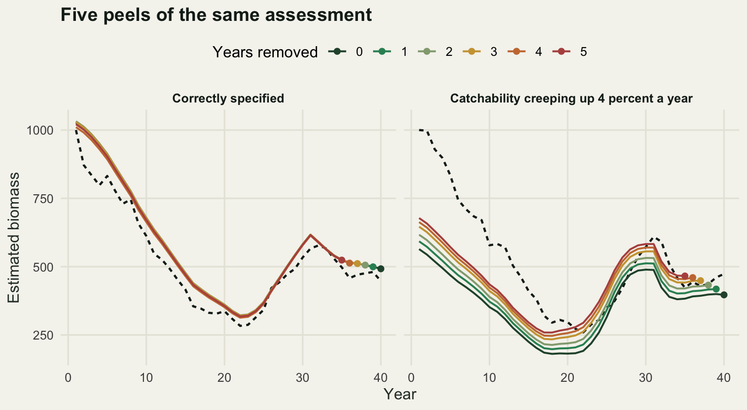
The correctly specified assessment gives a rho of -0.0008 and six lines that are hard to tell apart. The one fitted to an index whose catchability climbs by 4 per cent a year gives 0.1333 and the fan is obvious by eye. A reader can see the pattern here because the truth is drawn on the same axes, which is exactly what an analyst does not have. So the second half of the check is to find out what “near zero” means for a series of this length.
n_rho <- 30
n_rho_bad <- 12
set.seed(31)
rho_null <- sapply(seq_len(n_rho), function(i)
  mohn_rho(peel_fits(sim_stock(r_true, k_true, q_true, f_path, sig_obs, sig_proc))))
set.seed(41)
rho_alt <- sapply(seq_len(n_rho_bad), function(i)
  mohn_rho(peel_fits(sim_stock(r_true, k_true, q_true, f_path, sig_obs, sig_proc,
                               creep = gear_creep))))
round(c(replicates_null = n_rho, median_null = median(rho_null), sd_null = sd(rho_null),
        q05_null = quantile(rho_null, 0.05), q95_null = quantile(rho_null, 0.95)), 4)
replicates_null median_null sd_null q05_null.5% q95_null.95%
30.0000 -0.0017 0.0113 -0.0150 0.0128 round(c(replicates_creep = n_rho_bad, median_creep = median(rho_alt),
min_creep = min(rho_alt), max_creep = max(rho_alt),
flagged = mean(rho_alt > quantile(rho_null, 0.95))), 4)replicates_creep median_creep min_creep max_creep
12.0000 0.1139 0.0879 0.1508
flagged
1.0000 Across 30 correctly specified replicates the median rho is -0.0017 with a standard deviation of 0.0113, and the middle 90 per cent runs from -0.015 to 0.0128. Across 12 replicates with gear creep the smallest rho is 0.0879 and every one of the 12 lands above the 95th percentile of the correct case. On this operating model the diagnostic separates the two cases cleanly.
Read that with care. The scatter above is what a Schaefer stock with 5 per cent process deviations and a fixed fishing history produces; real assessments have age structure, changing selectivity and worse data, and their retrospective patterns scatter far more, which is why published guidance on acceptable rho values is expressed in tenths rather than hundredths. The number to compare your rho against is not a constant, it is a simulation of your own assessment. What the diagnostic tells you when it fires is also narrower than it looks: the fan says an assumption is wrong, and says nothing at all about which one. The pattern above would look much the same if natural mortality had been assumed too low, or if the catch had been under-reported by a growing margin. And the correctly specified panel is a reminder in the other direction, because a clean rho is a statement that the model is internally consistent as years are added, not that it is right.
Check (b): contrast, measured before the fit
The first post established that a monotonically declining series cannot separate the growth rate from the carrying capacity, so the yield estimate slides along a ridge. That was a result. Turned into a check it becomes a question an analyst can answer before fitting anything: how much does this index vary, and what does that variation buy?
The width of the interval is measured directly on a grid. Evaluate the negative log likelihood over growth rates and carrying capacities, keep the cells within two log-likelihood units of the best fit, and take the range of the implied yield across them. Three candidate contrast statistics go on the other axis: the fold range of the smoothed index, the standard deviation of its logarithm, and the largest rise the smoothed index makes above its own running low.
rgrid <- exp(seq(log(0.02), log(1), length.out = 95))
kgrid <- exp(seq(log(300), log(20000), length.out = 95))
gsurf <- expand.grid(r = rgrid, K = kgrid)
msy_cell <- gsurf$r * gsurf$K / 4

msy_span <- function(dat) {
  dv <- spm_nll(gsurf$r, gsurf$K, dat$catch, dat$cpue)
  dv <- 2 * (dv - min(dv))
  inn <- dv <= 4
  edge <- any(inn & (gsurf$r >= max(rgrid) * 0.999 | gsurf$K >= max(kgrid) * 0.999 |
                     gsurf$r <= min(rgrid) * 1.001 | gsurf$K <= min(kgrid) * 1.001))
  c(fold = max(msy_cell[inn]) / min(msy_cell[inn]), edge = as.numeric(edge))
}

smooth3 <- function(x) {
  s <- as.numeric(stats::filter(x, rep(1 / 3, 3), sides = 2))
  s[!is.na(s)]
}

index_stats <- function(idx) {
  s <- smooth3(idx)
  c(spread = max(s) / min(s), logsd = sd(log(s)), rebuild = max(s / cummin(s)))
}

n_series <- 60
set.seed(707)
contrast_tab <- do.call(rbind, lapply(seq_len(n_series), function(i) {
  n_up <- sample(8:34, 1)
  fmax <- runif(1, 0.12, 0.40)
  uu <- exp(runif(1, log(0.06), log(1.9)))
  fp <- c(seq(0.02, fmax, length.out = n_up),
          seq(fmax, fmax * uu, length.out = nyr - n_up))
  dd <- sim_stock(r_true, k_true, q_true, fp, sig_obs, sig_proc)
  if (min(dd$biomass) < 0.04 * k_true) return(NULL)
  data.frame(t(index_stats(dd$cpue)), t(msy_span(dd)))
}))
round(c(series_drawn = n_series, series_kept = nrow(contrast_tab),
        hit_search_box = sum(contrast_tab$edge), median_fold = median(contrast_tab$fold),
        max_fold = max(contrast_tab$fold)), 3)
series_drawn series_kept hit_search_box median_fold max_fold
60.000 57.000 13.000 1.165 15.468 Each of the 60 fishing histories ramps effort up over a random number of years and then either keeps pushing or eases off, so the resulting indices span everything from a smooth one-way decline to a deep fish-down and rebuild. Three collapsed to under 4 per cent of carrying capacity and were dropped, leaving 57. In 13 of them the two-unit region ran into the edge of the search grid, so their yield intervals are lower bounds rather than measurements.
round(c(spearman_spread = cor(contrast_tab$spread, contrast_tab$fold, method = "spearman"),
        spearman_logsd = cor(contrast_tab$logsd, contrast_tab$fold, method = "spearman"),
        spearman_rebuild = cor(contrast_tab$rebuild, contrast_tab$fold, method = "spearman")), 3)
spearman_spread spearman_logsd spearman_rebuild
-0.396 -0.380 -0.805 quint <- function(x) cut(x, quantile(x, seq(0, 1, 0.2)), include.lowest = TRUE)
bin_table <- function(x) {
gr <- quint(x)
data.frame(mid = round(tapply(x, gr, median), 3),
fold = round(tapply(contrast_tab$fold, gr, median), 3),
n = as.numeric(table(gr)))
}
print(bin_table(contrast_tab$spread)) mid fold n
[1.69,2.34] 2.003 2.343 12
(2.34,3.39] 2.809 1.160 11
(3.39,4.8] 3.777 1.077 11
(4.8,6.58] 5.644 1.453 11
(6.58,18.4] 8.373 1.039 12print(bin_table(contrast_tab$rebuild)) mid fold n
[1.09,1.28] 1.206 3.270 12
(1.28,1.47] 1.340 1.524 11
(1.47,1.66] 1.575 1.160 11
(1.66,2.09] 1.849 1.070 11
(2.09,3.44] 2.678 1.016 12reb_lm <- lm(log(fold) ~ log(rebuild), contrast_tab)
round(c(slope = as.numeric(coef(reb_lm)[2]), rsq = summary(reb_lm)$r.squared,
rebuild_at_fold_2 = as.numeric(exp((log(2) - coef(reb_lm)[1]) / coef(reb_lm)[2])),
rebuild_at_fold_1_5 = as.numeric(exp((log(1.5) - coef(reb_lm)[1]) / coef(reb_lm)[2]))), 3) slope rsq rebuild_at_fold_2 rebuild_at_fold_1_5
-1.192 0.300 1.383 1.760 stat_levels <- c("Index range: max / min", "Largest rise above a running low")
cmp <- rbind(
data.frame(stat = contrast_tab$spread, fold = contrast_tab$fold,
edge = contrast_tab$edge, which_stat = stat_levels[1]),
data.frame(stat = contrast_tab$rebuild, fold = contrast_tab$fold,
edge = contrast_tab$edge, which_stat = stat_levels[2]))
cmp$which_stat <- factor(cmp$which_stat, levels = stat_levels)
med_line <- do.call(rbind, lapply(stat_levels, function(nm) {
z <- cmp[cmp$which_stat == nm, ]
gr <- quint(z$stat)
data.frame(stat = as.numeric(tapply(z$stat, gr, median)),
fold = as.numeric(tapply(z$fold, gr, median)), which_stat = nm)
}))
med_line$which_stat <- factor(med_line$which_stat, levels = stat_levels)
ggplot(cmp, aes(stat, fold)) +
geom_hline(yintercept = 2, colour = te_pal$clay, linetype = "22", linewidth = 0.6) +
geom_point(aes(shape = factor(edge)), colour = te_pal$forest, size = 2, alpha = 0.85) +
geom_line(data = med_line, colour = te_pal$gold, linewidth = 0.9) +
geom_point(data = med_line, colour = te_pal$gold, size = 2.4) +
facet_wrap(~which_stat, scales = "free_x") +
scale_x_log10() + scale_y_log10() +
scale_shape_manual(values = c(16, 1), name = NULL, labels = c("bounded", "at grid edge")) +
labs(x = "Contrast statistic, smoothed index",
y = "MSY interval, fold range", title = "Not all contrast is the kind that pays") +
theme_te() +
theme(legend.position = "top",
strip.text = element_text(colour = te_pal$ink, face = "bold"))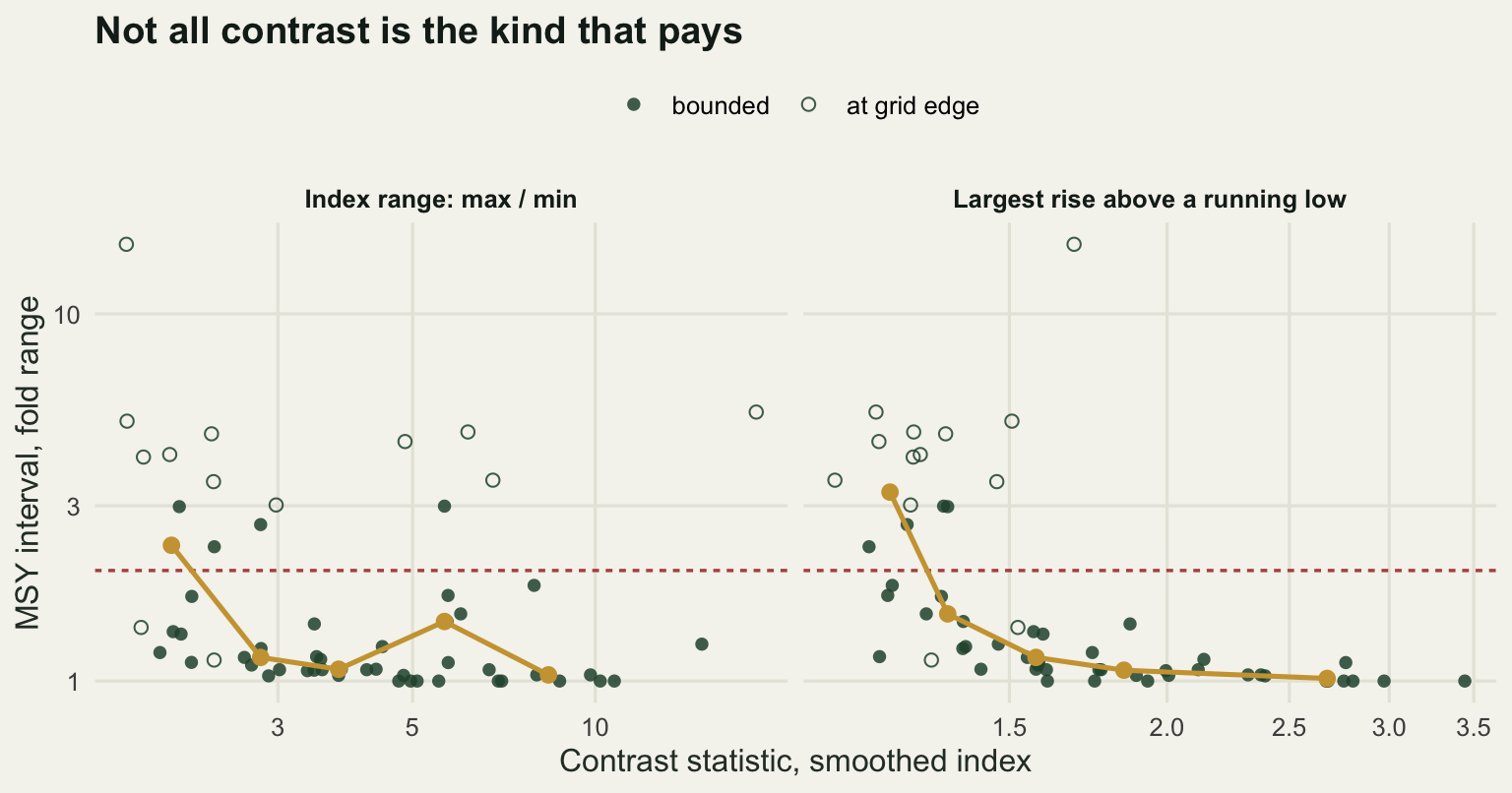
The statistic everyone quotes is one of the two weak ones. The rank correlation between the fold range of the index and the width of the yield interval is -0.396, the standard deviation of the log index is similarly weak at -0.380, and the binned medians of the range are not even monotone. On this run the fourth of the five groups has a median interval of 1.453, wider than the third at 1.077 and wider than the group with the widest index ranges of all at 1.039. The reason is the one-way trip. An index that falls by a factor of ten and never comes back has a huge range and tells you almost nothing about production at low biomass, which is the quantity that separates the growth rate from the carrying capacity.
The statistic that works is the rise: the largest factor by which the smoothed index climbs above its own running low. Its rank correlation with the interval width is -0.805, the strongest of the three, and the binned medians drop from end to end, from 3.27 in the fifth of series that barely rise at all to 1.016 in the fifth that rise most. Fitting the width on a log-log scale gives a slope of -1.192 with an R-squared of 0.3, and solving that line for an interval of a factor of two puts the threshold at a rise of 1.383 in this set of series. Below that, which is to say when the index never climbs more than about 40 per cent above its running low, the two-unit interval on yield is wider than a factor of two, and the assessment is choosing its answer from a family of nearly equally likely ones. That is a check you can run on your own index this afternoon, with no fitting at all.
The R-squared of 0.3 is worth staring at, because it means the prediction is loose. A series with a rise of 1.5 might still come back well determined, or might not. The check tells you which side of the line you are on, not what your interval will be, and the same shape of problem shows up whenever a short series is asked for a rate: the tutorial on detecting density dependence hits it in the bias of the autoregressive coefficient, where the fix is a bootstrap rather than a better optimiser.
Check (c): the assumed parameters, priced
A production model has no natural mortality in it. Mortality still gets in, through the back door, because the growth rate is the one parameter an index rarely determines, so in practice it is fixed or given a tight prior from life history. A common shortcut sets the fishing mortality at maximum sustainable yield to a fraction of natural mortality, which under Schaefer means the growth rate is proportional to it. We take the growth rate as 1.6 times the assumed natural mortality, fix it, and estimate the carrying capacity alone. The second standing assumption is the gear creep correction: the analyst deflates the index by an assumed percentage a year before fitting. The truth here is a natural mortality of 0.2 and creep of 2 per cent a year.
deflate <- function(dat, aa) {
  dd <- dat
  dd$cpue <- dat$cpue / (1 + aa)^(dat$year - 1)
  dd
}

fit_fixed <- function(dat, rr) {
  op <- optimize(function(lk) spm_nll(rr, exp(lk), dat$catch, dat$cpue),
                 c(log(300), log(20000)), tol = 1e-9)
  kk <- exp(op$minimum)
  bio <- as.vector(project_biomass(rr, kk, dat$catch)$bio)
  c(K = kk, msy = rr * kk / 4, depletion = bio[length(bio)] / kk,
    terminal = bio[length(bio)])
}

r_from_m <- function(mm) 1.6 * mm

set.seed(3007)
d_creepy <- sim_stock(r_true, k_true, q_true, f_path, sig_obs, sig_proc, creep = creep_true)
m_seq <- seq(0.12, 0.28, by = 0.02)
a_seq <- seq(0, 0.04, by = 0.005)
sweep_tab <- do.call(rbind, lapply(m_seq, function(mm) {
  do.call(rbind, lapply(a_seq, function(aa) {
    z <- fit_fixed(deflate(d_creepy, aa), r_from_m(mm))
    data.frame(M = mm, creep = aa, msy = z["msy"], depletion = z["depletion"])
  }))
}))
m_only <- sweep_tab[sweep_tab$creep == creep_true, ]
a_only <- sweep_tab[sweep_tab$M == m_true, ]

round(c(true_M = m_true, true_creep = creep_true, true_MSY = r_true * k_true / 4,
        true_depletion = d_creepy$biomass[nyr] / k_true,
        base_MSY = a_only$msy[a_only$creep == creep_true],
        base_depletion = a_only$depletion[a_only$creep == creep_true]), 4)
true_M true_creep true_MSY true_depletion base_MSY
0.2000 0.0200 80.0000 0.5091 74.1049
base_depletion
0.4007 round(c(M_sweep_MSY_fold = max(m_only$msy) / min(m_only$msy),
creep_sweep_MSY_fold = max(a_only$msy) / min(a_only$msy),
joint_MSY_fold = max(sweep_tab$msy) / min(sweep_tab$msy),
M_sweep_depletion_span = diff(range(m_only$depletion)),
creep_sweep_depletion_span = diff(range(a_only$depletion)),
joint_depletion_span = diff(range(sweep_tab$depletion))), 4) M_sweep_MSY_fold creep_sweep_MSY_fold
1.1959 1.0620
joint_MSY_fold M_sweep_depletion_span
1.3017 0.0339
creep_sweep_depletion_span joint_depletion_span
0.2549 0.3535 kprof <- exp(seq(log(300), log(20000), length.out = 4000))
nll_prof <- spm_nll(rep(r_true, length(kprof)), kprof, d_creepy$catch, d_creepy$cpue)
kin <- kprof[2 * (nll_prof - min(nll_prof)) <= 4]
dep_in <- sapply(kin, function(kk) {
bb <- as.vector(project_biomass(r_true, kk, d_creepy$catch)$bio)
bb[nyr] / kk
})
round(c(model_MSY_lo = r_true * min(kin) / 4, model_MSY_hi = r_true * max(kin) / 4,
model_MSY_fold = max(kin) / min(kin), model_depletion_lo = min(dep_in),
model_depletion_hi = max(dep_in), model_depletion_span = diff(range(dep_in))), 4) model_MSY_lo model_MSY_hi model_MSY_fold
74.6087 82.6096 1.1072
model_depletion_lo model_depletion_hi model_depletion_span
0.4259 0.5776 0.1517 round(c(MSY_log_ratio = log(max(sweep_tab$msy) / min(sweep_tab$msy)) /
log(max(kin) / min(kin)),
depletion_ratio = diff(range(sweep_tab$depletion)) / diff(range(dep_in))), 3) MSY_log_ratio depletion_ratio
2.589 2.331 n_mc <- 40
set.seed(451)
mc_tab <- do.call(rbind, lapply(seq_len(n_mc), function(i) {
dd <- sim_stock(r_true, k_true, q_true, f_path, sig_obs, sig_proc, creep = creep_true)
good <- fit_fixed(deflate(dd, creep_true), r_true)
naive <- fit_fixed(dd, r_true)
data.frame(msy = good["msy"], depletion = good["depletion"],
err = log(good["terminal"] / dd$biomass[nyr]),
err_naive = log(naive["terminal"] / dd$biomass[nyr]))
}))
round(c(replicates = n_mc,
noise_MSY_fold = as.numeric(quantile(mc_tab$msy, 0.95) / quantile(mc_tab$msy, 0.05)),
noise_depletion_span = as.numeric(diff(quantile(mc_tab$depletion, c(0.05, 0.95)))),
biomass_error_sd = sd(mc_tab$err),
biomass_bias_correct = exp(median(mc_tab$err)),
biomass_bias_naive = exp(median(mc_tab$err_naive)),
naive_bias_percent = 100 * (exp(median(mc_tab$err_naive)) - 1),
msy_error_sd = sd(log(mc_tab$msy / (r_true * k_true / 4)))), 4) replicates noise_MSY_fold noise_depletion_span
40.0000 1.1866 0.1711
biomass_error_sd biomass_bias_correct biomass_bias_naive
0.1688 0.9478 1.3427
naive_bias_percent msy_error_sd
34.2750 0.0580 quantity_levels <- c("Estimated MSY", "Estimated current depletion")
sw_long <- rbind(
data.frame(M = sweep_tab$M, creep = sweep_tab$creep, value = sweep_tab$msy,
quantity = quantity_levels[1]),
data.frame(M = sweep_tab$M, creep = sweep_tab$creep, value = sweep_tab$depletion,
quantity = quantity_levels[2]))
sw_long$quantity <- factor(sw_long$quantity, levels = quantity_levels)
bands <- data.frame(quantity = factor(quantity_levels, levels = quantity_levels),
ymin = c(r_true * min(kin) / 4, min(dep_in)),
ymax = c(r_true * max(kin) / 4, max(dep_in)))
truths <- data.frame(quantity = factor(quantity_levels, levels = quantity_levels),
yv = c(r_true * k_true / 4, d_creepy$biomass[nyr] / k_true))
ggplot(sw_long, aes(M, value, colour = creep, group = creep)) +
geom_rect(data = bands, aes(ymin = ymin, ymax = ymax, xmin = -Inf, xmax = Inf),
inherit.aes = FALSE, fill = te_pal$sage, alpha = 0.3) +
geom_hline(data = truths, aes(yintercept = yv), colour = te_pal$ink,
linetype = "22", linewidth = 0.6) +
geom_line(linewidth = 0.8) +
facet_wrap(~quantity, scales = "free_y") +
scale_colour_gradient(low = te_pal$green, high = te_pal$clay,
name = "Assumed gear creep") +
labs(x = "Assumed natural mortality M",
y = NULL, title = "What the two standing assumptions are worth") +
theme_te() +
theme(legend.position = "top",
strip.text = element_text(colour = te_pal$ink, face = "bold"))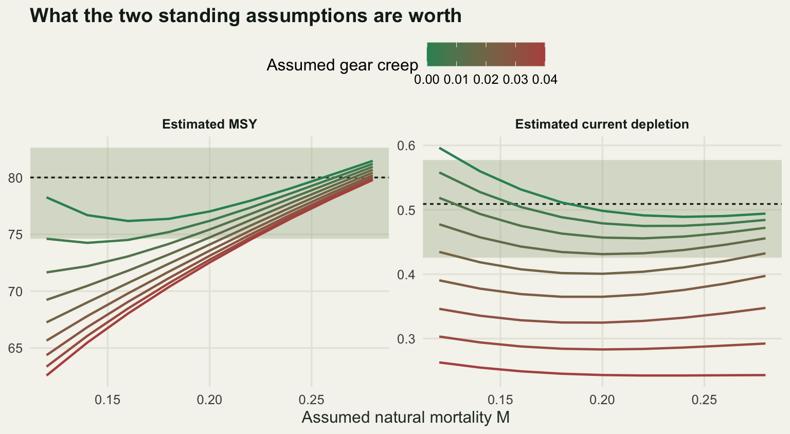
The ranking depends on which number you came for, and that is the result. Sweeping natural mortality from 0.12 to 0.28, a range no reviewer would object to, moves the yield estimate by a factor of 1.1959 and the depletion estimate by 0.0339. Sweeping the assumed gear creep from zero to 4 per cent a year moves the yield by a factor of only 1.062, and the depletion estimate by 0.2549, which is more than half of the distance from a healthy stock to a collapsed one. The same model, the same data: natural mortality moves the target more than the creep correction does, and the creep correction moves the status more than natural mortality does.
Both of those spreads should be set against the interval the model itself reports. With the assumptions pinned at the truth, the two-unit interval runs from 74.6087 to 82.6096 in yield and from 0.4259 to 0.5776 in depletion. The joint assumption sweep is 2.589 times wider than that on the yield, measured on the log scale, and 2.331 times wider on the depletion. Sampling noise, from 40 replicate datasets fitted with the assumptions correct, gives a 5th to 95th percentile yield range of a factor of 1.1866 and a depletion span of 0.1711, so on the yield the noise and the natural mortality assumption are worth about the same, and on the status the creep assumption is worth more than either.
The point of the arithmetic is not that assessments are useless. It is that the interval an assessment prints is a conditional interval, and the condition is that the fixed parameters were right. Anyone quoting one without the sweep beside it is quoting the smaller of two numbers.
One measurement from that block is used again below. An assessment that ignores a real gear creep of 2 per cent a year overestimates current biomass by 34.275 per cent at the end of the series, with the correctly specified version sitting at 0.9478 of the truth and a log error standard deviation of 0.1688.
Check (d): the control rule under estimation error
An assessment is an input to a decision. The check that matters is therefore not whether the fit is good but whether the fishery survives the rule that reads it, and the honest way to ask that is a closed loop: a true stock that keeps running, an assessment made each year with the errors we just measured, a control rule that turns the estimate into a catch, and feedback for as long as a management plan lives.
The assessment inside the loop is emulated rather than refitted, because refitting a likelihood inside 400 replicates of 50 years is minutes of compute for no extra realism. Its error is the one measured in check (c): a lognormal deviation with a log standard deviation of 0.1688, carried forward with an autocorrelation of 0.76, because successive annual assessments share almost all of their data and their errors do not reset. The biased variant multiplies the estimate by the factor of 1.3427 measured above.
Three rules compete. Constant fishing mortality takes a fixed fraction of the estimated biomass every year. Constant catch fixes a quota and holds it. The cut-off rule is the constant fishing mortality rule with a ramp: full fishing mortality above 0.4 of carrying capacity, falling linearly to zero at 0.1. The stock starts at 0.25 of carrying capacity, which is also the limit reference point, so the risk metric is the probability that the stock is below the limit at any point in the fifty years, and a rule that rebuilds cleanly scores near zero.
sig_est <- sd(mc_tab$err)
phi_est <- 0.76
bias_naive <- exp(median(mc_tab$err_naive))
f_target <- r_true / 2
b_start <- 0.25; b_limit <- 0.25; cut_off <- 0.10; b_trigger <- 0.40
n_proj <- 50; n_rep <- 400

close_loop <- function(rule, tac = 0, bias = 1, nrep = n_rep) {
  yld <- numeric(nrep); low <- logical(nrep)
  vary <- numeric(nrep); fin <- numeric(nrep)
  for (j in seq_len(nrep)) {
    bio <- b_start * k_true
    ee <- rnorm(1, 0, sig_est)
    got <- numeric(n_proj)
    hit <- FALSE
    for (i in seq_len(n_proj)) {
      ee <- phi_est * ee + sqrt(1 - phi_est^2) * rnorm(1, 0, sig_est)
      bhat <- bio * exp(ee) * bias
      cc <- switch(rule,
                   constant_f = f_target * bhat,
                   constant_catch = tac,
                   cutoff = f_target * bhat *
                     min(1, max(0, (bhat / k_true - cut_off) / (b_trigger - cut_off))))
      cc <- min(cc, 0.9 * bio)
      got[i] <- cc
      bio <- max((bio + production(bio, r_true, k_true) - cc) *
                   exp(rnorm(1, -sig_proc^2 / 2, sig_proc)), 1e-3)
      if (bio < b_limit * k_true) hit <- TRUE
    }
    yld[j] <- mean(got); low[j] <- hit; fin[j] <- bio / k_true
    vary[j] <- mean(abs(diff(got))) / mean(got)
  }
  c(yield = median(yld), risk = mean(low), catch_cv = median(vary),
    final_depletion = median(fin))
}

tac_seq <- seq(20, 80, by = 5)
rule_label <- c(constant_f = "constant F", cutoff = "cut-off rule",
                constant_catch = "constant catch")
one_run <- function(rule_id, tac, bias) {
  stopifnot(rule_id %in% names(rule_label))
  set.seed(2026)
  data.frame(rule_id = rule_id, rule = as.character(rule_label[rule_id]),
             tac = tac, bias = bias,
             t(close_loop(rule_id, tac = ifelse(is.na(tac), 0, tac), bias = bias)))
}
mse_tab <- do.call(rbind, lapply(c(1, bias_naive), function(bs) rbind(
  one_run("constant_f", NA, bs),
  one_run("cutoff", NA, bs),
  do.call(rbind, lapply(tac_seq, function(tc) one_run("constant_catch", tc, bs))))))
mse_tab$assessment <- ifelse(mse_tab$bias > 1.001, "biased", "unbiased")

round(c(projection_years = n_proj, replicates = n_rep, start_depletion = b_start,
        limit_reference_point = b_limit, cut_off = cut_off, trigger = b_trigger,
        F_target = f_target,
        assessment_error_sd = sig_est, assessment_autocorrelation = phi_est,
        bias_multiplier = bias_naive), 4)
projection_years replicates
50.0000 400.0000
start_depletion limit_reference_point
0.2500 0.2500
cut_off trigger
0.1000 0.4000
F_target assessment_error_sd
0.1600 0.1688
assessment_autocorrelation bias_multiplier
0.7600 1.3427 print(cbind(mse_tab[is.na(mse_tab$tac), c("rule", "assessment")],
round(mse_tab[is.na(mse_tab$tac),
c("yield", "risk", "catch_cv", "final_depletion")], 3))) rule assessment yield risk catch_cv final_depletion
1 constant F unbiased 71.996 0.130 0.109 0.491
2 cut-off rule unbiased 72.706 0.018 0.134 0.494
16 constant F biased 65.464 0.840 0.112 0.316
17 cut-off rule biased 67.669 0.693 0.156 0.337cc_un <- mse_tab[mse_tab$rule_id == "constant_catch" & mse_tab$assessment == "unbiased", ]
print(round(cc_un[, c("tac", "yield", "risk", "catch_cv")], 3)) tac yield risk catch_cv
3 20 20.000 0.000 0.000
4 25 25.000 0.000 0.000
5 30 30.000 0.010 0.000
6 35 35.000 0.022 0.000
7 40 40.000 0.055 0.000
8 45 45.000 0.142 0.000
9 50 50.000 0.282 0.000
10 55 55.000 0.515 0.000
11 60 39.612 0.775 0.031
12 65 17.595 0.953 0.075
13 70 14.130 1.000 0.101
14 75 12.414 1.000 0.123
15 80 11.326 1.000 0.144risk_f <- mse_tab$risk[mse_tab$rule_id == "constant_f" & mse_tab$assessment == "unbiased"]
matched <- cc_un[cc_un$risk <= risk_f, ]
round(c(constant_F_risk = risk_f, best_matched_constant_catch_yield = max(matched$yield),
constant_F_yield = mse_tab$yield[mse_tab$rule_id == "constant_f" &
mse_tab$assessment == "unbiased"],
cutoff_yield = mse_tab$yield[mse_tab$rule_id == "cutoff" &
mse_tab$assessment == "unbiased"],
yield_given_up_percent = 100 * (1 - max(matched$yield) /
mse_tab$yield[mse_tab$rule_id == "constant_f" &
mse_tab$assessment == "unbiased"])), 3) constant_F_risk best_matched_constant_catch_yield
0.130 40.000
constant_F_yield cutoff_yield
71.996 72.706
yield_given_up_percent
44.441 assess_levels <- c("Unbiased assessment", "Biomass overestimated by a third")
mse_tab$panel <- factor(ifelse(mse_tab$assessment == "unbiased",
assess_levels[1], assess_levels[2]), levels = assess_levels)
cc_line <- mse_tab[mse_tab$rule_id == "constant_catch", ]
pts <- mse_tab[is.na(mse_tab$tac), ]
ggplot(cc_line, aes(risk, yield)) +
geom_line(colour = te_pal$sage, linewidth = 0.9) +
geom_point(aes(colour = rule), size = 2) +
geom_point(data = pts, aes(colour = rule), size = 4) +
facet_wrap(~panel) +
scale_colour_manual(values = c("constant F" = te_pal$forest,
"cut-off rule" = te_pal$gold,
"constant catch" = te_pal$clay), name = NULL) +
labs(x = "Probability the stock falls below the limit",
y = "Median annual yield", title = "Yield against risk over fifty years") +
theme_te() +
theme(legend.position = "top",
strip.text = element_text(colour = te_pal$ink, face = "bold"))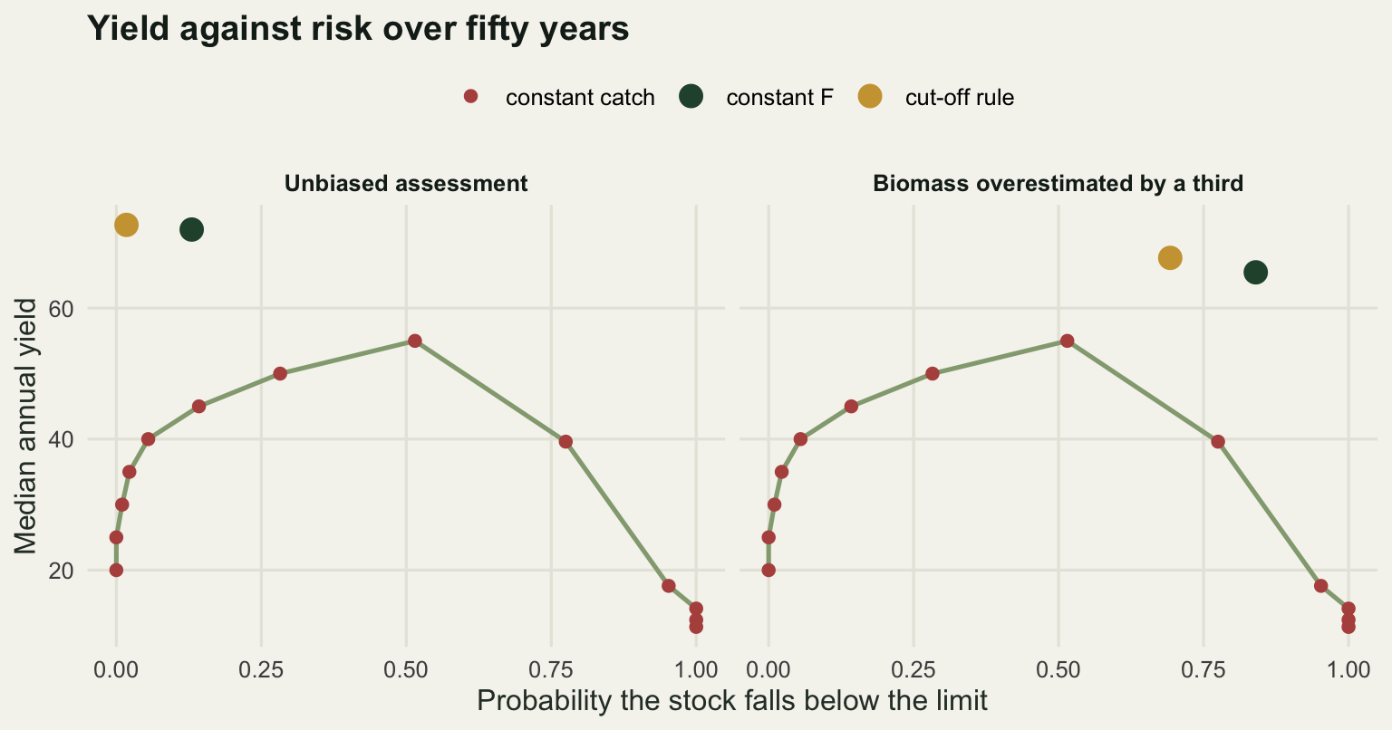
Under an unbiased assessment the constant fishing mortality rule takes a median 71.996 a year and drops below the limit in 0.13 of replicates. The cut-off rule takes 72.706 and drops below the limit in 0.018 of them. That was not the expected result. The cut-off was supposed to buy safety at a cost in yield, and it did not cost any: protecting the stock at low biomass lets it rebuild sooner, and over fifty years the extra production more than pays for the catch given up early. What the cut-off does cost is stability. The median year-to-year change in the catch rises from 0.109 of the mean catch to 0.134, and that is a real price for a fleet with fixed costs, just not the price the textbook version of this comparison advertises.
Constant catch is the dangerous one, and the curve shows why. It never touches the feedback rules. At a quota of 55 it yields 55 and hits the limit in 0.515 of replicates; at any quota whose risk matches the constant fishing mortality rule, the best it can do is a yield of 40, which is 44.441 per cent less than the feedback rule earns at the same risk. Its one virtue is visible in the same table: the year-to-year change in the catch is exactly zero until the quota gets large enough that the stock cannot supply it. A rule that does not read the assessment cannot be misled by it, and cannot be corrected by it either. That is also why the constant catch curve is identical in both panels of the figure: the bias never reaches it. A manager setting a quota from a biased assessment simply picks a point further to the right along the same curve without knowing it.
The second panel is the one to take away. Feed the same three rules an assessment that overestimates biomass by a third, which is what check (c) measured for a 2 per cent a year gear creep that nobody corrected, and the cut-off rule’s probability of breaching the limit goes from 0.018 to 0.693. The constant fishing mortality rule goes from 0.13 to 0.84. Neither rule changed. The rule that tested as safe is safe against sampling noise in the assessment, not against a mistake in it, and no amount of tuning the ramp will fix a biomass estimate that is a third too high. Yield falls too, from 71.996 to 65.464 and from 72.706 to 67.669, so the biased assessment does not even buy short-term catch: it takes fish from a stock that cannot replace them.
What none of these checks can see
Each of the four checks compares the assessment against the data it was fitted to, or against the model family it was built from. That is the boundary, and it is worth stating without softening.
A regime shift that changes productivity is invisible to all four. If the growth rate halves because the plankton community reorganised, the retrospective peels will eventually notice something is wrong, but only after years of advice have been issued at the old level, and the diagnostic will not say what changed. Stock structure is invisible: if what is being assessed is two populations mixing on the fishing grounds, every check above can pass while one component is fished to nothing under a total biomass that looks stable. Under-reported catch is invisible in a particular way, because the catch series enters the model as data rather than as an observation with error, so a systematic shortfall is absorbed into the estimated production and comes back out as an optimistic yield. An ecosystem interaction that moves natural mortality, a predator recovering or a fishery removing one, shifts the very quantity check (c) treats as a fixed assumption to be swept over.
An assessment can produce a retrospective pattern near zero, a well conditioned likelihood, an index with plenty of the right kind of contrast, and a control rule that tests well in a closed loop, and still be managing a fiction. The checks measure internal consistency. They do not measure whether the model is about the right fish.
Where to go next
The cluster closes here. The first post left an honest limit at the likelihood ridge: a yield estimate whose two-unit interval spanned a factor of three on a one-way trip. The second left one at steepness, a parameter that recruitment data barely constrain and that moves the target fishing mortality a long way. The third left one at hyperstability, an index that keeps looking healthy while the stock thins out. This post’s contribution is the fourth: even when all three are handled well, the answer is conditional on assumptions the data cannot test, and the decision rule reading it can convert a modest bias into a large probability of collapse.
For the same estimate-then-decide loop in a conservation setting, where the currency is persistence rather than yield and the projection horizon is longer than the data, extinction risk and population viability analysis runs the equivalent exercise: a fitted population model, a decision that depends on it, and a careful account of what the projection is entitled to say.
References
Mohn R 1999 ICES Journal of Marine Science 56(4):473-488 (10.1006/jmsc.1999.0481)
Hurtado-Ferro F, Szuwalski CS, Valero JL, Anderson SC, Cunningham CJ, Johnson KF, Licandeo R, McGilliard CR, Monnahan CC, Muradian ML, Ono K, Vert-pre KA, Whitten AR, Punt AE 2015 ICES Journal of Marine Science 72(1):99-110 (10.1093/icesjms/fsu198)
Punt AE, Butterworth DS, de Moor CL, De Oliveira JAA, Haddon M 2016 Fish and Fisheries 17(2):303-334 (10.1111/faf.12104)
Vert-pre KA, Amoroso RO, Jensen OP, Hilborn R 2013 Proceedings of the National Academy of Sciences 110(5):1779-1784 (10.1073/pnas.1214879110)
Hilborn R, Walters CJ 1992 Quantitative Fisheries Stock Assessment. Chapman and Hall, ISBN 978-0-412-02271-5