Stock-recruitment and reference points

Beverton-Holt and Ricker curves in steepness form, per-recruit fishery reference points in base R, and how much of Fmsy is data and how much is assumption.

A stock assessment ends with a number that a manager can act on: a target fishing mortality, a biomass below which the fishery should close. The sibling tutorial on surplus production models gets to MSY from a biomass dynamics model with no ages in it at all, which is honest about what a catch and index series can support. This post opens the age structure and asks what the extra machinery buys. Recruits enter at age one, grow, mature, and die at a rate nobody measured; the fishery removes a share of each age class.

Two pieces of arithmetic sit between the life history and the reference point. The first is the stock-recruitment relationship: how many recruits a given spawning biomass produces. The second is the per-recruit calculation: how much spawning biomass and how much yield a single recruit generates over its lifetime at a given fishing mortality. Reference points come out of those two, and the second one is much better behaved than the first.

Everything here is base R plus ggplot2. Growth comes from a von Bertalanffy curve; if you want the fitting side of that, the tutorial on fitting growth curves with nls covers it, including why the asymptote is an extrapolation. Here the curve is taken as given so the attention stays on what happens downstream. What gets measured: how much the recruitment data actually say about steepness, how much steepness moves Fmsy, and which of the three standing assumptions (steepness, natural mortality, functional form) moves the answer most.

library(ggplot2)

te_pal <- list(forest = "#275139", green = "#2f8f63", sage = "#93a87f",
               clay = "#b5534e", gold = "#cda23f", line = "#dad9ca",
               ink = "#16241d", paper = "#f5f4ee")

theme_te <- function() {
  theme_minimal(base_size = 12) +
    theme(panel.grid.minor = element_blank(),
          panel.grid.major = element_line(colour = "#e7e6dc"),
          plot.background = element_rect(fill = "#f5f4ee", colour = NA),
          panel.background = element_rect(fill = "#f5f4ee", colour = NA),
          plot.title = element_text(face = "bold", colour = te_pal$ink),
          axis.title = element_text(colour = "#2c3a31"))
}

Steepness, and where the equilibrium sits

Start with a cohort. Forty age classes, a von Bertalanffy length at age, a cubic length-weight relation, logistic maturity and logistic selectivity. These are the only biology in the model, and none of them is estimated here.

ages <- 1:40
linf <- 80; kvb <- 0.18; age0 <- -0.5
wa <- 9.0e-6; wb <- 3

len_age <- linf * (1 - exp(-kvb * (ages - age0)))
wt_age <- wa * len_age^wb
mat_age <- 1 / (1 + exp(-(ages - 4.0) / 0.8))
sel_age <- 1 / (1 + exp(-(ages - 3.0) / 0.7))
m_base <- 0.2

print(data.frame(age = ages[1:8],
                 cm = round(len_age[1:8], 1),
                 kg = round(wt_age[1:8], 3),
                 mature = round(mat_age[1:8], 3),
                 selected = round(sel_age[1:8], 3)))

  age   cm    kg mature selected
1   1 18.9 0.061  0.023    0.054
2   2 29.0 0.219  0.076    0.193
3   3 37.4 0.471  0.223    0.500
4   4 44.4 0.788  0.500    0.807
5   5 50.3 1.144  0.777    0.946
6   6 55.2 1.511  0.924    0.986
7   7 59.3 1.873  0.977    0.997
8   8 62.7 2.216  0.993    0.999

Fish are selected by the gear a year or so before they mature, which is the usual and uncomfortable arrangement. Now run one recruit through its life with no fishing and add up the spawning biomass it produces. That total is the virgin spawning biomass per recruit, written phi0, and it is the hinge on which everything else turns.

per_recruit <- function(fm, mnat = m_base) {
  zz <- mnat + fm * sel_age
  nn <- numeric(length(zz))
  nn[1] <- 1
  for (a in seq_along(zz)[-1]) nn[a] <- nn[a - 1] * exp(-zz[a - 1])
  c(spr = sum(nn * mat_age * wt_age),
    ypr = sum(nn * wt_age * (fm * sel_age / zz) * (1 - exp(-zz))),
    tip = nn[40] * mat_age[40] * wt_age[40])
}

spr_of <- function(fm, mnat = m_base) unname(per_recruit(fm, mnat)["spr"])
ypr_of <- function(fm, mnat = m_base) unname(per_recruit(fm, mnat)["ypr"])

phi0 <- spr_of(0)
cat("virgin spawning biomass per recruit:", round(phi0, 3), "kg\n")

virgin spawning biomass per recruit: 6.037 kg

cat("share contributed by the oldest age class:",
    signif(unname(per_recruit(0)["tip"]) / phi0, 3), "\n")

share contributed by the oldest age class: 0.000312 

cat("replacement slope when unfished (recruits per kg):", round(1 / phi0, 4), "\n")

replacement slope when unfished (recruits per kg): 0.1656 

One recruit yields 6.037 kg of spawning biomass over its life. The oldest age class contributes 0.000312 of that, so truncating at forty ages costs nothing. Turn phi0 upside down and you get the replacement line: an unfished population needs 0.1656 recruits per kilogram of spawning biomass to stay where it is.

Steepness is defined against that virgin state. It is the share of virgin recruitment produced when spawning biomass is knocked down to 20 per cent of virgin. Both the Beverton-Holt and the Ricker function can be written in terms of steepness h and virgin recruitment R0, and that is the form managers use, because h is bounded and comparable across stocks in a way that the raw curve parameters are not.

r0_virgin <- 1000
ssb0 <- r0_virgin * phi0

sr_bh <- function(ssb, h, r0 = r0_virgin, ph0 = phi0) {
  4 * h * r0 * ssb / (r0 * ph0 * (1 - h) + ssb * (5 * h - 1))
}

sr_rk <- function(ssb, h, r0 = r0_virgin, ph0 = phi0) {
  (ssb / ph0) * (5 * h)^(1.25 * (1 - ssb / (r0 * ph0)))
}

hset <- c(0.3, 0.5, 0.7, 0.9)
chk <- data.frame(
  steepness = hset,
  bh_at_20pc = round(sr_bh(0.2 * ssb0, hset) / r0_virgin, 4),
  rk_at_20pc = round(sr_rk(0.2 * ssb0, hset) / r0_virgin, 4),
  bh_at_virgin = round(sr_bh(ssb0, hset) / r0_virgin, 4),
  rk_at_virgin = round(sr_rk(ssb0, hset) / r0_virgin, 4),
  comp_bh = round(4 * hset / (1 - hset), 3),
  comp_rk = round((5 * hset)^1.25, 3))
print(chk)

  steepness bh_at_20pc rk_at_20pc bh_at_virgin rk_at_virgin comp_bh comp_rk
1       0.3        0.3        0.3            1            1   1.714   1.660
2       0.5        0.5        0.5            1            1   4.000   3.144
3       0.7        0.7        0.7            1            1   9.333   4.787
4       0.9        0.9        0.9            1            1  36.000   6.554

The definition checks out numerically: at 20 per cent of virgin spawning biomass both functions return exactly h times virgin recruitment, and both pass through virgin recruitment at virgin biomass. The last two columns are the compensation ratio, the slope of the curve at the origin divided by the replacement slope. This is where the two functions part company. At h = 0.7 Beverton-Holt implies 9.333 times replacement at low biomass while Ricker implies 4.787; at h = 0.9 the gap is 36 against 6.554. The same steepness means very different things about how hard a depleted stock pushes back.

Equilibrium is the point where the recruitment curve crosses the replacement line for the fishing mortality in force. Fishing steepens the replacement line, because a fished recruit produces less spawning biomass, so fewer recruits per kilogram are needed to hold station. Both functions have a closed-form equilibrium, which is worth writing out rather than solving numerically.

eq_bh <- function(fm, h, mnat = m_base) {
  ph <- spr_of(fm, mnat); ph0 <- spr_of(0, mnat)
  ssb <- max(r0_virgin * (4 * h * ph - ph0 * (1 - h)) / (5 * h - 1), 0)
  rec <- if (ssb > 0) ssb / ph else 0
  c(ssb = ssb, rec = rec, yield = rec * ypr_of(fm, mnat))
}

eq_rk <- function(fm, h, mnat = m_base) {
  ph <- spr_of(fm, mnat); ph0 <- spr_of(0, mnat)
  frac <- 1 - log(ph0 / ph) / (1.25 * log(5 * h))
  ssb <- max(frac * r0_virgin * ph0, 0)
  rec <- if (ssb > 0) ssb / ph else 0
  c(ssb = ssb, rec = rec, yield = rec * ypr_of(fm, mnat))
}

f_demo <- 0.15
cat("replacement slope at F = 0.15:", round(1 / spr_of(f_demo), 4), "\n")

replacement slope at F = 0.15: 0.4051 

cat("spawning potential ratio at that F:", round(spr_of(f_demo) / phi0, 4), "\n")

spawning potential ratio at that F: 0.4089 

eqtab <- data.frame(
  steepness = hset,
  bh_ssb = round(vapply(hset, function(h)
    unname(eq_bh(f_demo, h)["ssb"]) / ssb0, 0), 3),
  rk_ssb = round(vapply(hset, function(h)
    unname(eq_rk(f_demo, h)["ssb"]) / ssb0, 0), 3),
  min_spr_bh = round((1 - hset) / (4 * hset), 3))
print(eqtab)

  steepness bh_ssb rk_ssb min_spr_bh
1       0.3  0.000  0.000      0.583
2       0.5  0.212  0.219      0.250
3       0.7  0.338  0.429      0.107
4       0.9  0.392  0.524      0.028

At a fishing mortality of 0.15 the replacement slope rises from 0.1656 to 0.4051, because a recruit now delivers only 0.4089 of the spawning biomass it would have delivered unfished. Under Beverton-Holt that same fishing mortality leaves the stock at 0.338 of virgin if h = 0.7 and wipes it out if h = 0.3. The last column says why: for Beverton-Holt there is a minimum spawning potential ratio below which no equilibrium exists, equal to (1 - h) / (4h), and at h = 0.3 that threshold is 0.583. Fishing to a spawning potential ratio of 0.409 is inside the safe zone for a resilient stock and past the point of no return for an unresilient one.

sfrac <- seq(0.002, 1.2, by = 0.004)

curve_df <- do.call(rbind, lapply(hset, function(h) {
  rbind(data.frame(model = "Beverton-Holt", h = h, sfrac = sfrac,
                   rfrac = sr_bh(sfrac * ssb0, h) / r0_virgin),
        data.frame(model = "Ricker", h = h, sfrac = sfrac,
                   rfrac = sr_rk(sfrac * ssb0, h) / r0_virgin))
}))
curve_df$hlab <- paste("h =", curve_df$h)

rep_df <- do.call(rbind, lapply(c("Beverton-Holt", "Ricker"), function(mm)
  data.frame(model = mm, which_line = c("unfished", "at F = 0.15"),
             slope = c(1, phi0 / spr_of(f_demo)))))

eq_pts <- do.call(rbind, lapply(hset, function(h) {
  aa <- eq_bh(f_demo, h); bb <- eq_rk(f_demo, h)
  rbind(data.frame(model = "Beverton-Holt", sfrac = aa["ssb"] / ssb0,
                   rfrac = aa["rec"] / r0_virgin),
        data.frame(model = "Ricker", sfrac = bb["ssb"] / ssb0,
                   rfrac = bb["rec"] / r0_virgin))
}))
eq_pts <- eq_pts[eq_pts$sfrac > 0, ]

p1 <- ggplot(curve_df, aes(sfrac, rfrac)) +
  geom_abline(data = rep_df,
              aes(slope = slope, intercept = 0, linetype = which_line),
              colour = te_pal$ink, linewidth = 0.4) +
  geom_line(aes(colour = hlab), linewidth = 0.8) +
  geom_point(data = eq_pts, colour = te_pal$clay, size = 2.4) +
  facet_wrap(~ model) +
  scale_colour_manual(values = c(te_pal$clay, te_pal$gold,
                                 te_pal$green, te_pal$forest), name = NULL) +
  scale_linetype_manual(values = c("dashed", "dotted"), name = NULL) +
  scale_x_continuous(breaks = c(0, 0.25, 0.5, 0.75, 1)) +
  coord_cartesian(ylim = c(0, 1.35)) +
  labs(title = "Steepness is the whole recruitment assumption",
       x = "Spawning biomass (share of virgin)",
       y = "Recruitment (share of virgin)") +
  theme_te() +
  theme(legend.position = "bottom")
print(p1)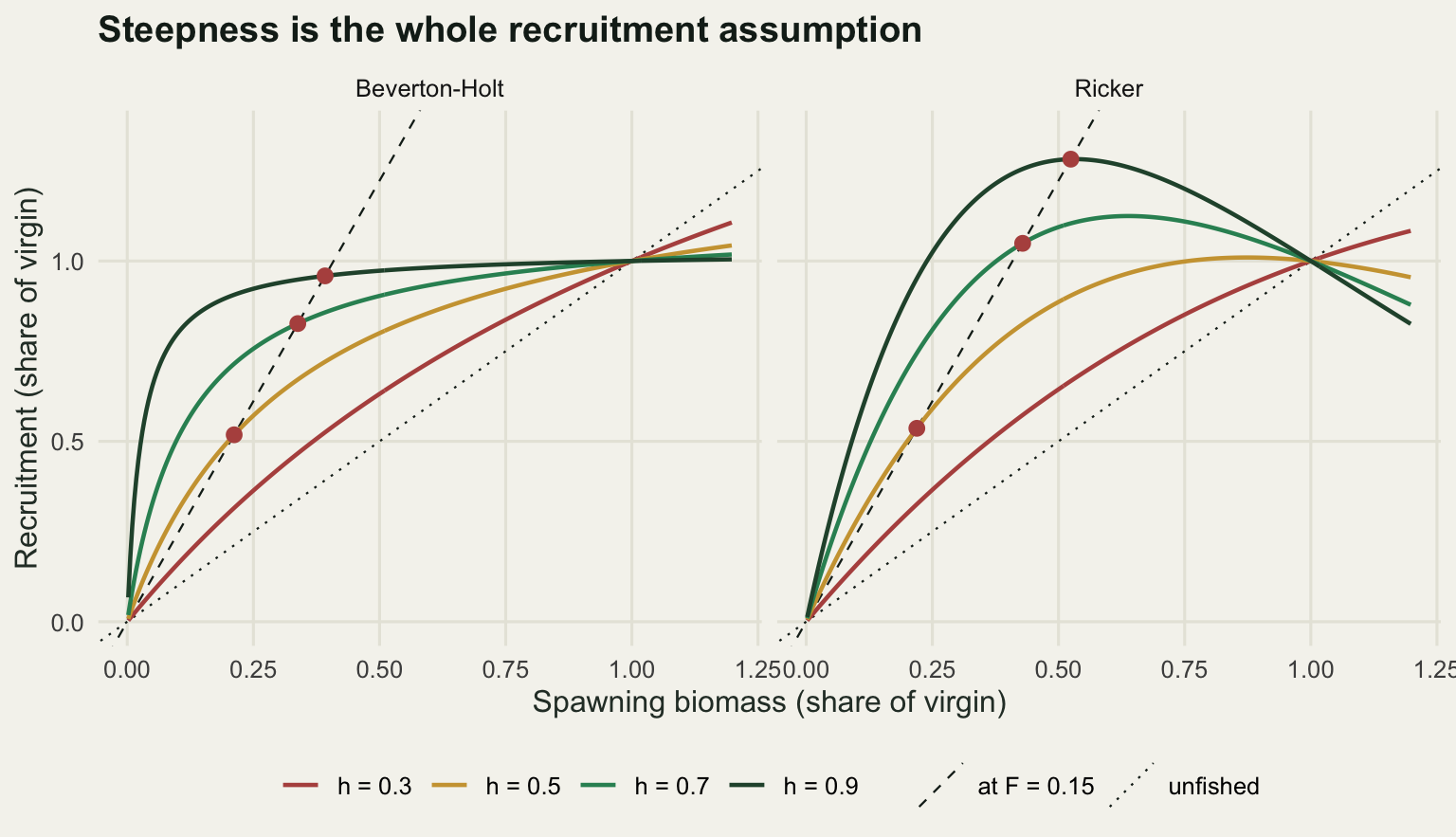

Figure 1: Beverton-Holt and Ricker recruitment curves at four steepness values, with the unfished replacement line and the replacement line at F = 0.15. Points mark the equilibria at F = 0.15.

Per-recruit reference points

The per-recruit side needs no recruitment curve at all. Run one recruit through the cohort at a given fishing mortality, add up spawning biomass and add up catch weight with the Baranov equation. The spawning potential ratio is spawning biomass per recruit divided by phi0.

f_grid <- seq(0, 1.2, by = 0.005)
grid_df <- data.frame(fm = f_grid,
                      ypr = vapply(f_grid, ypr_of, 0),
                      spr = vapply(f_grid, spr_of, 0) / phi0)
print(grid_df[grid_df$fm %in% c(0, 0.05, 0.1, 0.15, 0.2, 0.3, 0.5, 1.0), ],
      row.names = FALSE, digits = 4)

   fm    ypr     spr
 0.00 0.0000 1.00000
 0.05 0.2044 0.70470
 0.10 0.3047 0.52576
 0.15 0.3556 0.40892
 0.20 0.3810 0.32825
 0.30 0.3966 0.22675
 0.50 0.3825 0.12962
 1.00 0.3258 0.05373

Three reference points come off these two curves. Fmax is where yield per recruit peaks. F0.1 is where the slope of the yield-per-recruit curve has fallen to a tenth of its slope at the origin, a deliberately conservative stopping rule from an era with no recruitment model to hand. F40%SPR is where the spawning potential ratio falls to 0.4.

slope_ypr <- function(fm, mnat = m_base, eps = 1e-5) {
  lo <- max(fm - eps, 0)
  (ypr_of(fm + eps, mnat) - ypr_of(lo, mnat)) / (fm + eps - lo)
}

f01_of <- function(mnat = m_base) {
  s_org <- slope_ypr(0, mnat)
  uniroot(function(x) slope_ypr(x, mnat) - 0.1 * s_org, c(1e-4, 3))$root
}

fmax_of <- function(mnat = m_base)
  optimise(function(x) ypr_of(x, mnat), c(1e-4, 5), maximum = TRUE)$maximum

fspr_of <- function(target, mnat = m_base)
  uniroot(function(x) spr_of(x, mnat) / spr_of(0, mnat) - target, c(1e-6, 5))$root

f01 <- f01_of(); fmx <- fmax_of(); f40 <- fspr_of(0.4)

cat("slope of yield per recruit at the origin:", round(slope_ypr(0), 3), "\n")

slope of yield per recruit at the origin: 5.815 

cat("F0.1 =", round(f01, 4), " slope there over slope at origin =",
    round(slope_ypr(f01) / slope_ypr(0), 4), "\n")

F0.1 = 0.1645  slope there over slope at origin = 0.1 

cat("Fmax =", round(fmx, 4), " slope there =", signif(slope_ypr(fmx), 2), "\n")

Fmax = 0.3153  slope there = 1.1e-05 

cat("F40%SPR =", round(f40, 4), " spawning potential ratio there =",
    round(spr_of(f40) / phi0, 4), "\n")

F40%SPR = 0.1547  spawning potential ratio there = 0.4 

cat("yield per recruit at F0.1:", round(ypr_of(f01), 4),
    " at Fmax:", round(ypr_of(fmx), 4),
    " ratio:", round(ypr_of(f01) / ypr_of(fmx), 4), "\n")

yield per recruit at F0.1: 0.3649  at Fmax: 0.3968  ratio: 0.9196 

cat("spawning potential ratio at F0.1:", round(spr_of(f01) / phi0, 4),
    " at Fmax:", round(spr_of(fmx) / phi0, 4), "\n")

spawning potential ratio at F0.1: 0.3826  at Fmax: 0.2157 

cat("F0.1 divided by F40%SPR:", round(f01 / f40, 4), "\n")

F0.1 divided by F40%SPR: 1.0628 

The verification is in the second and third lines: at F0.1 the slope really is 0.1 of the slope at the origin, and at Fmax the slope really is zero to five decimal places. F0.1 is 0.1645 and Fmax is 0.3153, so the conservative rule sits at roughly half the yield-maximising rate and retains 0.9196 of the peak yield per recruit, giving up about eight per cent to get there. What it buys is spawning biomass: 0.3826 of virgin per recruit rather than 0.2157.

F40%SPR is 0.1547, which is 1.063 times smaller than F0.1. For this life history the two reference points, arrived at from different directions and different decades, are the same number to within six per cent. That is a coincidence of this parameter set rather than a general result, but it happens often enough that the two are frequently treated as interchangeable.

pan_lv <- c("Yield per recruit (kg)", "Spawning potential ratio")

pr_long <- rbind(
  data.frame(fm = grid_df$fm, value = grid_df$ypr, panel = pan_lv[1]),
  data.frame(fm = grid_df$fm, value = grid_df$spr, panel = pan_lv[2]))
pr_long$panel <- factor(pr_long$panel, levels = pan_lv)

mark_df <- rbind(
  data.frame(panel = pan_lv[1], fm = c(f01, fmx), rp = c("F0.1", "Fmax")),
  data.frame(panel = pan_lv[2], fm = c(f01, f40), rp = c("F0.1", "F40%SPR")))
mark_df$panel <- factor(mark_df$panel, levels = pan_lv)

p2 <- ggplot(pr_long, aes(fm, value)) +
  geom_vline(data = mark_df, aes(xintercept = fm, colour = rp),
             linewidth = 0.6, linetype = "dashed") +
  geom_line(colour = te_pal$forest, linewidth = 0.9) +
  facet_wrap(~ panel, scales = "free_y") +
  scale_colour_manual(values = c(te_pal$clay, te_pal$gold, te_pal$green),
                      name = NULL) +
  coord_cartesian(xlim = c(0, 0.8)) +
  labs(title = "Per-recruit curves and the points taken off them",
       x = "Fishing mortality F", y = NULL) +
  theme_te() +
  theme(legend.position = "bottom")
print(p2)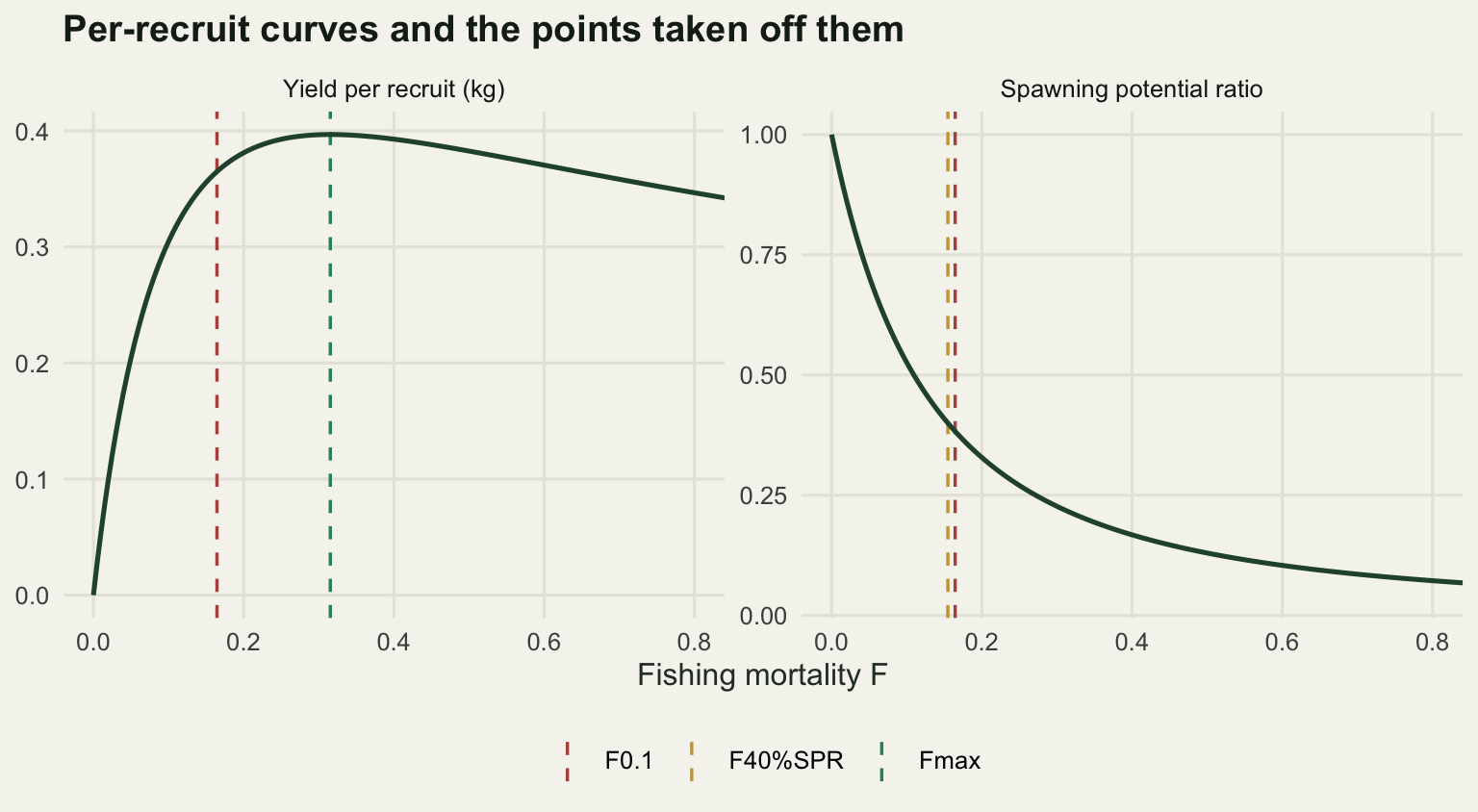

Figure 2: Yield per recruit and spawning potential ratio against fishing mortality, with F0.1, Fmax and F40%SPR marked.

Steepness is barely estimable, and it sets Fmsy

Fmsy needs both halves: the per-recruit arithmetic to convert fishing mortality into yield and spawning biomass per recruit, and the recruitment curve to say how many recruits an equilibrium spawning biomass produces. So Fmsy depends on steepness, and the question is whether a recruitment series can pin steepness down.

Simulate one. Thirty years of spawning biomass and recruitment, a stock fished down gradually from near virgin, lognormal recruitment noise with a standard deviation of 0.6 on the log scale. That noise level is ordinary for a marine fish; if anything it is on the tame side.

set.seed(20260818)

sim_series <- function(nyr, h_true, sigma, dep_hi, dep_lo) {
  dep <- seq(dep_hi, dep_lo, length.out = nyr) * exp(rnorm(nyr, 0, 0.06))
  ssb <- dep * ssb0
  data.frame(ssb = ssb, rec = sr_bh(ssb, h_true) * exp(rnorm(nyr, 0, sigma)))
}

dat_real <- sim_series(30, 0.7, 0.6, 0.90, 0.35)
dat_good <- sim_series(60, 0.7, 0.25, 0.95, 0.06)

cat("realistic series: years =", nrow(dat_real),
    " depletion from", round(max(dat_real$ssb) / ssb0, 3),
    "to", round(min(dat_real$ssb) / ssb0, 3),
    " contrast ratio", round(max(dat_real$ssb) / min(dat_real$ssb), 2), "\n")

realistic series: years = 30  depletion from 0.9 to 0.347  contrast ratio 2.59 

cat("recruitment coefficient of variation:",
    round(sd(dat_real$rec) / mean(dat_real$rec), 3), "\n")

recruitment coefficient of variation: 0.628 

cat("favourable series: years =", nrow(dat_good),
    " depletion from", round(max(dat_good$ssb) / ssb0, 3),
    "to", round(min(dat_good$ssb) / ssb0, 3), "\n")

favourable series: years = 60  depletion from 1.011 to 0.054 

Fit steepness by maximum likelihood with virgin recruitment free and the residual standard deviation concentrated out, then profile over a grid of steepness values. The truth is 0.7.

nll_at_h <- function(h, dd, srfun) {
  fn <- function(lr0) {
    pred <- srfun(dd$ssb, h, exp(lr0), phi0)
    if (any(!is.finite(pred)) || any(pred <= 0)) return(1e6)
    resid_log <- log(dd$rec) - log(pred)
    nrow(dd) / 2 * log(sum(resid_log^2) / nrow(dd))
  }
  optimise(fn, c(log(50), log(50000)))$objective
}

h_grid <- seq(0.21, 0.99, by = 0.01)
prof_real <- vapply(h_grid, nll_at_h, 0, dd = dat_real, srfun = sr_bh)
prof_good <- vapply(h_grid, nll_at_h, 0, dd = dat_good, srfun = sr_bh)
supported <- function(pv) h_grid[pv - min(pv) < 1.92]

cat("realistic: best h =", h_grid[which.min(prof_real)],
    " supported range", round(min(supported(prof_real)), 2), "to",
    round(max(supported(prof_real)), 2),
    " width", round(diff(range(supported(prof_real))), 3), "\n")

realistic: best h = 0.47  supported range 0.26 to 0.99  width 0.73 

cat("favourable: best h =", h_grid[which.min(prof_good)],
    " supported range", round(min(supported(prof_good)), 2), "to",
    round(max(supported(prof_good)), 2),
    " width", round(diff(range(supported(prof_good))), 3), "\n")

favourable: best h = 0.67  supported range 0.6 to 0.74  width 0.14 

cat("realistic penalty for h = 0.3 versus best:",
    round(prof_real[h_grid == 0.3] - min(prof_real), 3),
    " for h = 0.9:", round(prof_real[h_grid == 0.9] - min(prof_real), 3), "\n")

realistic penalty for h = 0.3 versus best: 0.663  for h = 0.9: 0.584 

The realistic series puts the maximum at 0.47 when the truth is 0.7, and the interval within 1.92 log-likelihood units runs from 0.26 to 0.99: a width of 0.73 on a parameter whose entire admissible range is a little wider than that. Assuming h = 0.3 costs 0.663 log-likelihood units against the best fit and assuming h = 0.9 costs 0.584. Neither penalty here would be noticed in a model comparison. Thirty years of recruitment data have, in effect, left steepness open.

The second series shows what it would take. Sixty years, a quarter of the recruitment noise, and the stock fished down to 0.054 of virgin: the profile then closes to a width of 0.14 and lands on 0.67. So steepness is estimable in principle. It needs a long series, a quiet stock and a depletion history that most managers would call a failure.

prof_df <- rbind(
  data.frame(h = h_grid, dev = prof_real - min(prof_real),
             case = "30 years, noisy, narrow contrast"),
  data.frame(h = h_grid, dev = prof_good - min(prof_good),
             case = "60 years, quiet, wide contrast"))

p3 <- ggplot(prof_df, aes(h, dev, colour = case)) +
  geom_hline(yintercept = 1.92, linetype = "dotted", colour = te_pal$ink) +
  geom_vline(xintercept = 0.7, linetype = "dashed", colour = te_pal$sage) +
  geom_line(linewidth = 0.9) +
  scale_colour_manual(values = c(te_pal$clay, te_pal$forest), name = NULL) +
  coord_cartesian(ylim = c(0, 6)) +
  labs(title = "What the recruitment data know about steepness",
       x = "Steepness h",
       y = "Profile negative log-likelihood above its minimum") +
  theme_te() +
  theme(legend.position = "bottom")
print(p3)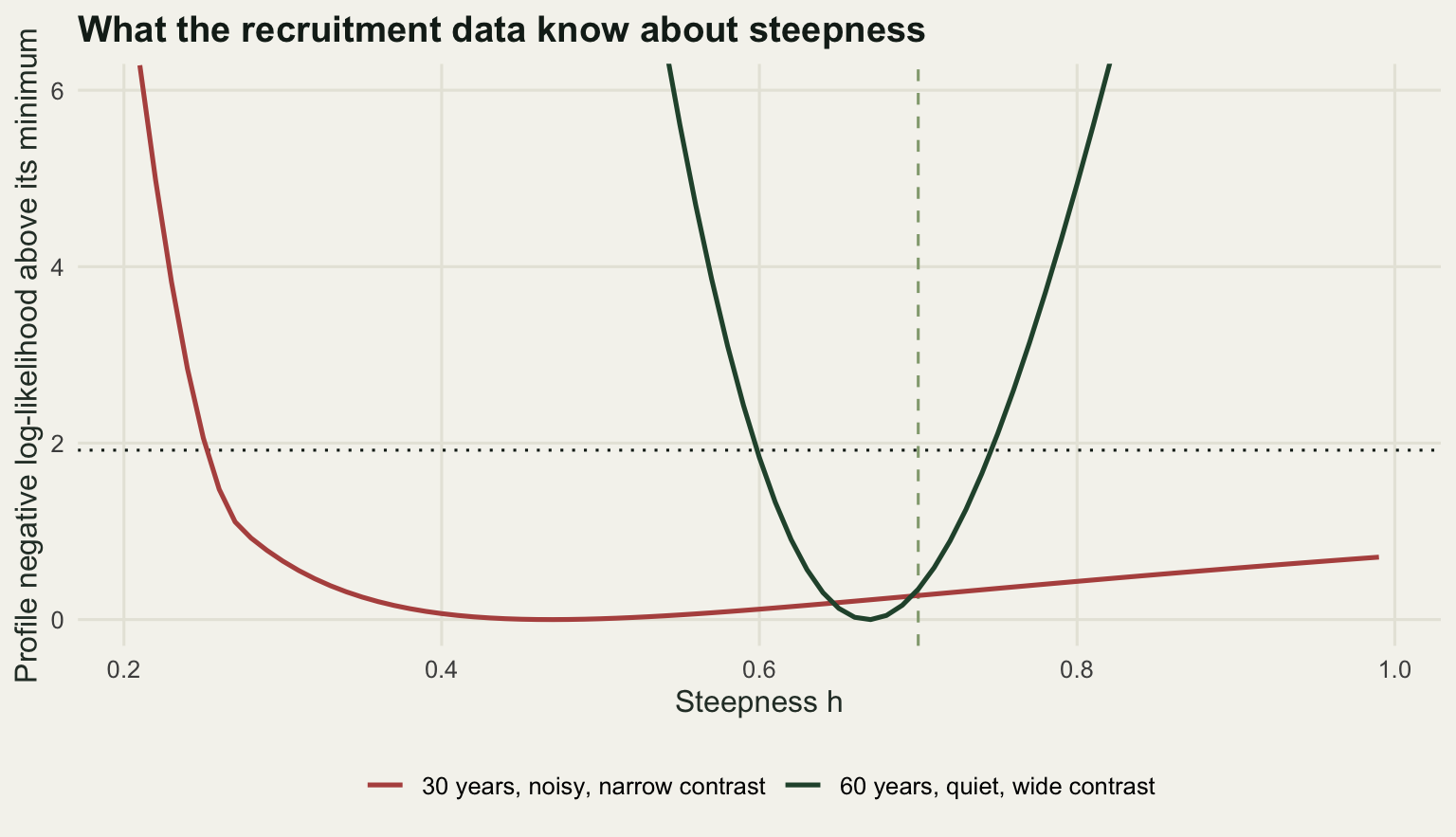

Figure 3: Profile negative log-likelihood for steepness under two data scenarios; the dotted line is 1.92 units above the minimum and the dashed vertical line marks the true value.

Now the other side of the asymmetry. Hold the life history fixed and sweep steepness across the range the data failed to exclude.

fmsy_of <- function(h, fun = eq_bh, mnat = m_base) {
  coarse <- seq(0.005, 1.5, by = 0.005)
  yy <- vapply(coarse, function(x) unname(fun(x, h, mnat)["yield"]), 0)
  best <- coarse[which.max(yy)]
  fine <- seq(max(best - 0.005, 1e-4), best + 0.005, by = 0.0005)
  fine[which.max(vapply(fine, function(x) unname(fun(x, h, mnat)["yield"]), 0))]
}

h_ref <- c(0.3, 0.4, 0.5, 0.6, 0.7, 0.8, 0.9)
ref_tab <- data.frame(h = h_ref)
ref_tab$Fmsy <- round(vapply(h_ref, fmsy_of, 0), 4)
ref_tab$Bmsy_B0 <- round(vapply(seq_along(h_ref), function(i)
  unname(eq_bh(ref_tab$Fmsy[i], h_ref[i])["ssb"]) / ssb0, 0), 3)
ref_tab$MSY <- round(vapply(seq_along(h_ref), function(i)
  unname(eq_bh(ref_tab$Fmsy[i], h_ref[i])["yield"]), 0), 1)
ref_tab$SPR_at_Fmsy <- round(vapply(ref_tab$Fmsy, function(x)
  spr_of(x) / phi0, 0), 3)
print(ref_tab, row.names = FALSE)

   h   Fmsy Bmsy_B0   MSY SPR_at_Fmsy
 0.3 0.0365   0.447  94.7       0.770
 0.4 0.0675   0.412 161.2       0.633
 0.5 0.0975   0.377 213.2       0.533
 0.6 0.1275   0.347 256.4       0.456
 0.7 0.1595   0.318 294.4       0.391
 0.8 0.1965   0.289 329.1       0.333
 0.9 0.2430   0.257 362.5       0.277

cat("Fmsy at h = 0.9 divided by Fmsy at h = 0.3:",
    round(ref_tab$Fmsy[7] / ref_tab$Fmsy[1], 2), "\n")

Fmsy at h = 0.9 divided by Fmsy at h = 0.3: 6.66 

cat("Bmsy/B0 at h = 0.3 divided by that at h = 0.9:",
    round(ref_tab$Bmsy_B0[1] / ref_tab$Bmsy_B0[7], 2), "\n")

Bmsy/B0 at h = 0.3 divided by that at h = 0.9: 1.74 

cat("MSY ratio across the same range:",
    round(ref_tab$MSY[7] / ref_tab$MSY[1], 2), "\n")

MSY ratio across the same range: 3.83 

Fmsy runs from 0.0365 to 0.2430 across a steepness range the likelihood surface here treats as essentially equivalent: a factor of 6.66. MSY itself changes by a factor of 3.83, and the biomass target Bmsy/B0 moves from 0.447 down to 0.257, a factor of 1.74. The asymmetry is plain in the two sets of numbers. Thirty years of recruitment data moved the steepness estimate hardly at all, and the choice between the values it could not separate moves the fishing mortality target by nearly sevenfold.

The last column is quietly interesting. The spawning potential ratio that corresponds to Fmsy runs from 0.770 at h = 0.3 down to 0.277 at h = 0.9, and it passes through 0.391 at h = 0.7. A 40 per cent target matches Fmsy only for a stock of moderate resilience; for a weak stock it is far too aggressive and for a strong one it leaves fish in the water.

What a per-recruit target buys, and what it does not

F0.1 and F40%SPR were computed above without reference to steepness. They cannot move when it changes, because it does not appear in the calculation. That is the whole appeal: they are estimable from growth, maturity, selectivity and natural mortality, none of which requires a recruitment series.

cons <- data.frame(h = h_ref)
cons$F01_over_Fmsy <- round(f01 / ref_tab$Fmsy, 2)
cons$ssb_at_F01 <- round(vapply(h_ref, function(h)
  unname(eq_bh(f01, h)["ssb"]) / ssb0, 0), 3)
cons$yield_share_F01 <- round(vapply(seq_along(h_ref), function(i)
  unname(eq_bh(f01, h_ref[i])["yield"]) / ref_tab$MSY[i], 0), 3)
cons$ssb_at_F40 <- round(vapply(h_ref, function(h)
  unname(eq_bh(f40, h)["ssb"]) / ssb0, 0), 3)
cons$yield_share_F40 <- round(vapply(seq_along(h_ref), function(i)
  unname(eq_bh(f40, h_ref[i])["yield"]) / ref_tab$MSY[i], 0), 3)
print(cons, row.names = FALSE)

   h F01_over_Fmsy ssb_at_F01 yield_share_F01 ssb_at_F40 yield_share_F40
 0.3          4.51      0.000           0.000      0.000           0.000
 0.4          2.44      0.012           0.072      0.040           0.223
 0.5          1.69      0.177           0.791      0.200           0.842
 0.6          1.29      0.259           0.964      0.280           0.980
 0.7          1.03      0.309           0.999      0.328           0.999
 0.8          0.84      0.341           0.989      0.360           0.981
 0.9          0.68      0.365           0.960      0.383           0.947

cat("F0.1 and F40%SPR are the same under every steepness:",
    round(f01, 4), round(f40, 4), "\n")

F0.1 and F40%SPR are the same under every steepness: 0.1645 0.1547 

This is where the measurement went somewhere I did not expect. At the assumed truth of h = 0.7, F0.1 is 1.03 times Fmsy and delivers 0.999 of MSY. As an MSY proxy it is close to perfect, which is presumably why it has survived fifty years of criticism. At h = 0.9 it is cautious, 0.68 of Fmsy, and the caution costs only 4 per cent of yield because the equilibrium yield curve is flat near its peak. At h = 0.5 it still returns 0.791 of MSY.

Then it falls off a cliff. At h = 0.4, F0.1 is 2.44 times Fmsy and equilibrium yield is 0.072 of MSY; at h = 0.3 it is 4.51 times Fmsy and the stock has no positive equilibrium at all. F40%SPR behaves the same way one notch later. So the per-recruit target is not safe in any absolute sense: it is safe across most of the steepness range and catastrophic at the bottom of it, and the data cannot tell you which end you are at. Fishing at a number you can estimate does not make the consequences of that number estimable.

fe_grid <- seq(0, 0.6, by = 0.005)
hpick <- h_ref[c(1, 3, 5, 7)]

eq_df <- do.call(rbind, lapply(hpick, function(h)
  data.frame(fm = fe_grid, h = h,
             yield = vapply(fe_grid, function(x)
               unname(eq_bh(x, h)["yield"]), 0))))
eq_df$hlab <- paste("h =", eq_df$h)

msy_pts <- data.frame(fm = ref_tab$Fmsy[c(1, 3, 5, 7)],
                      yield = ref_tab$MSY[c(1, 3, 5, 7)])

p4 <- ggplot(eq_df, aes(fm, yield, colour = hlab)) +
  geom_vline(xintercept = f01, linetype = "dashed", colour = te_pal$ink) +
  geom_line(linewidth = 0.9) +
  geom_point(data = msy_pts, aes(fm, yield), inherit.aes = FALSE,
             colour = te_pal$ink, size = 2.2) +
  scale_colour_manual(values = c(te_pal$clay, te_pal$gold, te_pal$green,
                                 te_pal$forest), name = NULL) +
  labs(title = "One fixed target, four different consequences",
       x = "Fishing mortality F", y = "Equilibrium yield (kg)") +
  theme_te() +
  theme(legend.position = "bottom")
print(p4)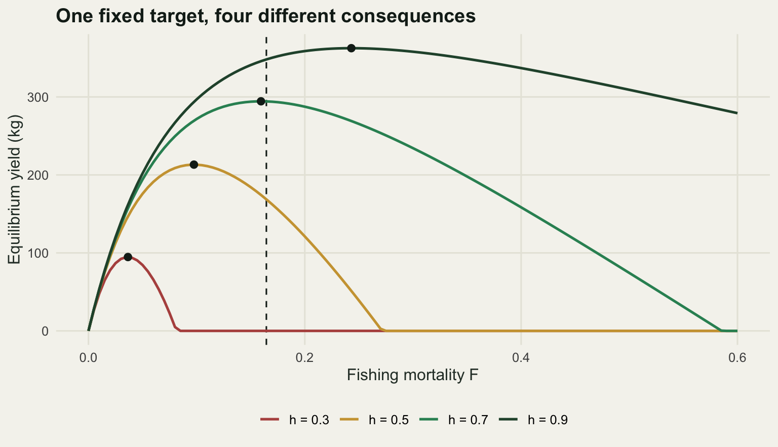

Figure 4: Equilibrium yield against fishing mortality under four steepness values. The dashed vertical line is F0.1, which does not move; dots mark Fmsy, which does.

Natural mortality and functional form

Steepness is not the only parameter that is assumed rather than estimated. Natural mortality is usually fixed from a life-history relationship or borrowed from a related stock, and it enters every one of these reference points. Sweep it over a range that no tagging study would rule out.

m_set <- c(0.15, 0.2, 0.25, 0.3)
m_tab <- data.frame(M = m_set)
m_tab$F01 <- round(vapply(m_set, f01_of, 0), 3)
m_tab$F40 <- round(vapply(m_set, function(x) fspr_of(0.4, x), 0), 3)
m_tab$Fmax <- round(vapply(m_set, fmax_of, 0), 3)
m_tab$Fmsy_h07 <- round(vapply(m_set, function(x) fmsy_of(0.7, eq_bh, x), 0), 3)
print(m_tab, row.names = FALSE)

    M   F01   F40  Fmax Fmsy_h07
 0.15 0.127 0.122 0.233    0.124
 0.20 0.164 0.155 0.315    0.160
 0.25 0.205 0.189 0.412    0.198
 0.30 0.250 0.225 0.527    0.239

cat("M doubles from", min(m_set), "to", max(m_set),
    "; F0.1 changes by a factor", round(m_tab$F01[4] / m_tab$F01[1], 2),
    ", F40%SPR by", round(m_tab$F40[4] / m_tab$F40[1], 2),
    ", Fmsy by", round(m_tab$Fmsy_h07[4] / m_tab$Fmsy_h07[1], 2), "\n")

M doubles from 0.15 to 0.3 ; F0.1 changes by a factor 1.97 , F40%SPR by 1.84 , Fmsy by 1.93 

cat("steepness triples from 0.3 to 0.9; F0.1 unchanged, Fmsy changes by",
    round(ref_tab$Fmsy[7] / ref_tab$Fmsy[1], 2), "\n")

steepness triples from 0.3 to 0.9; F0.1 unchanged, Fmsy changes by 6.66 

Doubling natural mortality moves F0.1 from 0.127 to 0.250, a factor of 1.97, and moves Fmsy at fixed steepness by 1.93. Every reference point scales with M in roughly the same way, which is the ranking worth carrying away. Against a tripling of steepness, F0.1 does not move at all and Fmsy moves by 6.66. So the per-recruit points are sensitive to M and immune to steepness, while Fmsy is sensitive to both and more sensitive to steepness than to M over these ranges. There is a partial consolation: because M scales all of them together, an error in M shifts the target and the yardstick in the same direction, which is not true of an error in steepness.

The third assumption is the shape of the curve itself. Fit both functions to the same thirty-year series and see whether the data prefer one.

prof_rk <- vapply(h_grid, nll_at_h, 0, dd = dat_real, srfun = sr_rk)
h_bh <- h_grid[which.min(prof_real)]
h_rk <- h_grid[which.min(prof_rk)]

cat("Beverton-Holt: best h =", h_bh, " negative log-likelihood",
    round(min(prof_real), 4), "\n")

Beverton-Holt: best h = 0.47  negative log-likelihood -16.6421 

cat("Ricker:        best h =", h_rk, " negative log-likelihood",
    round(min(prof_rk), 4), "\n")

Ricker:        best h = 0.46  negative log-likelihood -16.6767 

cat("difference in AIC (same parameter count):",
    round(2 * (min(prof_rk) - min(prof_real)), 3), "\n")

difference in AIC (same parameter count): -0.069 

fmsy_bh <- fmsy_of(h_bh, eq_bh)
fmsy_rk <- fmsy_of(h_rk, eq_rk)
cat("Fmsy under Beverton-Holt:", round(fmsy_bh, 3),
    " under Ricker:", round(fmsy_rk, 3), "\n")

Fmsy under Beverton-Holt: 0.089  under Ricker: 0.085 

cat("Bmsy/B0 under Beverton-Holt:",
    round(unname(eq_bh(fmsy_bh, h_bh)["ssb"]) / ssb0, 3),
    " under Ricker:", round(unname(eq_rk(fmsy_rk, h_rk)["ssb"]) / ssb0, 3), "\n")

Bmsy/B0 under Beverton-Holt: 0.387  under Ricker: 0.462 

cat("MSY under Beverton-Holt:", round(unname(eq_bh(fmsy_bh, h_bh)["yield"]), 1),
    " under Ricker:", round(unname(eq_rk(fmsy_rk, h_rk)["yield"]), 1), "\n")

MSY under Beverton-Holt: 198.7  under Ricker: 227.7 

The difference in AIC is 0.069, which is nothing: the data were generated by a Beverton-Holt curve and the Ricker fit is indistinguishable from it. At the same time the two fits disagree about the biomass target, 0.387 of virgin against 0.462, and about MSY, 198.7 against 227.7. The functional form is a third unidentified assumption with real consequences, and the fact that it was chosen by convention rather than by fit is not visible anywhere in the output.

Where the mortality rate itself comes from

Total mortality has been an input on this page rather than an output. m_base is 0.2 because it was written down, F is the dial, and Z is their sum. In an assessment with ages in it both usually arrive through a catch curve: a straight line fitted to log catch at age along the descending limb of a single year’s age composition. That needs no machinery beyond the cohort recursion already written above, and one assumption that rarely reaches the methods section, which is that every cohort in the sample recruited at the same strength.

Drop it and the algebra is two lines. If recruitment has been changing at a constant rate g per year, the cohort now aged a recruited a minus one years ago and enters the sample multiplied by exp(-g(a - 1)). On the log scale that factor is itself a straight line in age, so it lands in the slope and nowhere else, and the fitted line returns Z + g instead of Z. This is algebra rather than a measurement, and it is exact under four conditions: selectivity flat across the ages fitted, M and F and selectivity unchanged through time, recruitment log-linear across the span of the sample, and observation error additive on the log scale.

set.seed(20260815)

f_cc <- 0.20                    # the fishing mortality the fleet is actually exerting
cc_ages <- 6:20                 # fully selected, and still numerous
sel_flat <- ifelse(ages >= min(cc_ages), 1, sel_age)

caa_year <- function(g, fm = f_cc, mnat = m_base, sel = sel_age) {
  zz <- mnat + fm * sel
  nn <- numeric(length(zz)); nn[1] <- 1
  for (a in seq_along(zz)[-1]) nn[a] <- nn[a - 1] * exp(-zz[a - 1])
  nn <- nn * exp(-g * (ages - 1))
  nn * (fm * sel / zz) * (1 - exp(-zz))
}

fit_cc <- function(logc) {
  xx <- cc_ages - mean(cc_ages); yy <- logc - mean(logc)
  b <- sum(xx * yy) / sum(xx^2)
  c(Z = -b, r2 = (sum(xx * yy)^2 / sum(xx^2)) / sum(yy^2))
}

g_dec <- log(0.94)              # recruitment falling 6 per cent a year
g_set <- c(-0.15, -0.05, 0, 0.05, 0.15)

cc_det <- t(vapply(g_set, function(g) {
  a <- fit_cc(log(caa_year(g)[cc_ages]))
  b <- fit_cc(log(caa_year(g, sel = sel_flat)[cc_ages]))
  c(g = g, Z_plus_g = m_base + f_cc + g, Zhat = a["Z"],
    gap = a["Z"] - (m_base + f_cc + g), r2 = a["r2"],
    gap_flat = b["Z"] - (m_base + f_cc + g), r2_flat = b["r2"])
}, numeric(7)))
colnames(cc_det) <- c("g", "Z_plus_g", "Zhat", "gap", "r2", "gap_flat", "r2_flat")
print(signif(cc_det, 6))

         g Z_plus_g     Zhat          gap       r2     gap_flat r2_flat
[1,] -0.15     0.25 0.249498 -0.000502444 0.999990  0.00000e+00       1
[2,] -0.05     0.35 0.349498 -0.000502444 0.999995 -1.11022e-16       1
[3,]  0.00     0.40 0.399498 -0.000502444 0.999996 -5.55112e-17       1
[4,]  0.05     0.45 0.449498 -0.000502444 0.999997 -5.55112e-17       1
[5,]  0.15     0.55 0.549498 -0.000502444 0.999998 -1.11022e-16       1

cc_gap <- max(abs(cc_det[, "gap"]))
cc_gap_flat <- max(abs(cc_det[, "gap_flat"]))
cc_r2_zero <- min(cc_det[, "r2"])
cc_ferr_big <- max(abs(100 * (cc_det[, "Zhat"] - m_base - f_cc) / f_cc))

f_targets <- c(`F = 0.2` = 0.20, `F0.1` = f01, `F40%SPR` = f40)
cc_ferr <- vapply(f_targets, function(fm)
  100 * (unname(fit_cc(log(caa_year(g_dec, fm = fm)[cc_ages]))["Z"]) - m_base - fm) / fm, 0)
print(round(rbind(F_assumed = f_targets, F_error_per_cent = cc_ferr,
                  algebra_g_over_F = 100 * g_dec / f_targets), 3))

                 F = 0.2    F0.1 F40%SPR
F_assumed          0.200   0.164   0.155
F_error_per_cent -31.189 -37.921 -40.301
algebra_g_over_F -30.938 -37.624 -39.987

With selectivity forced flat across the fitted ages the identity holds to 1e-16 and the line is exact, so R-squared comes back as 1. The logistic selectivity of this post is still climbing at age six, so over ages 6 to 20 the fitted line misses Z + g by 0.000502, and misses by that same amount at every trend rate: the selectivity gap and the recruitment gap add rather than interact.

The second table is the one that reaches a decision. M is subtracted from the catch curve estimate to get F, and subtracting a constant does not shrink an error, so a bias of g in Z is a relative error of g over F in F. Recruitment falling 6 per cent a year puts F out by 31 per cent at F = 0.2, by 38 per cent at the F0.1 computed earlier, and by 40 per cent at F40%SPR. The more precautionary the target, the larger the relative error, because the same absolute bias in Z is set against a smaller F. Three assumptions have already been priced on this page: steepness, natural mortality, and the shape of the recruitment curve, the last of which left two very different biomass targets that the AIC comparison could not separate. This is a fourth, and it sits underneath the other three, because the M in m_base and the F a harvest rule compares against F0.1 both come off the same line.

Now separate the two things that can go wrong with that line. Observation error scatters the points around it; a recruitment trend tilts it. Vary both.

set.seed(20260816)

cc_mc <- function(nrep, g, sigma) {
  xx <- cc_ages - mean(cc_ages); mm <- length(cc_ages)
  Y <- log(caa_year(g)[cc_ages]) + matrix(rnorm(nrep * mm, 0, sigma), mm)
  Yc <- Y - rep(colMeans(Y), each = mm)
  sxy <- as.vector(crossprod(xx, Yc)); b <- sxy / sum(xx^2)
  r2 <- (sxy^2 / sum(xx^2)) / colSums(Yc^2)
  c(Z = mean(-b), Z_se = sd(b) / sqrt(nrep), r2 = mean(r2), r2_se = sd(r2) / sqrt(nrep))
}

sig_set <- c(0, 0.1, 0.2, 0.4, 0.8)
grid_cc <- expand.grid(sigma = sig_set, g = g_set)
grid_cc <- cbind(grid_cc,
                 t(mapply(function(g, s) cc_mc(4000, g, s), grid_cc$g, grid_cc$sigma)))
grid_cc$F_error <- 100 * (grid_cc$Z - m_base - f_cc) / f_cc

shape_cc <- function(col, d) {
  mm <- matrix(grid_cc[[col]], nrow = length(sig_set),
               dimnames = list(paste0("sigma=", sig_set), sprintf("g=%+.2f", g_set)))
  round(mm, d)
}
cat("mean R-squared\n"); print(shape_cc("r2", 4))

mean R-squared

          g=-0.15 g=-0.05 g=+0.00 g=+0.05 g=+0.15
sigma=0    1.0000  1.0000  1.0000  1.0000  1.0000
sigma=0.1  0.9926  0.9962  0.9971  0.9977  0.9985
sigma=0.2  0.9707  0.9848  0.9884  0.9909  0.9939
sigma=0.4  0.8925  0.9427  0.9554  0.9644  0.9758
sigma=0.8  0.6718  0.8016  0.8425  0.8710  0.9108

cat("\nestimated Z, the truth being 0.4\n"); print(shape_cc("Z", 3))

estimated Z, the truth being 0.4

          g=-0.15 g=-0.05 g=+0.00 g=+0.05 g=+0.15
sigma=0     0.249   0.349   0.399   0.449   0.549
sigma=0.1   0.250   0.350   0.400   0.449   0.549
sigma=0.2   0.250   0.349   0.399   0.450   0.550
sigma=0.4   0.250   0.350   0.400   0.449   0.549
sigma=0.8   0.249   0.349   0.400   0.450   0.551

cat("\nerror in F, per cent, the truth being 0.2\n"); print(shape_cc("F_error", 1))

error in F, per cent, the truth being 0.2

          g=-0.15 g=-0.05 g=+0.00 g=+0.05 g=+0.15
sigma=0     -75.3   -25.3    -0.3    24.7    74.7
sigma=0.1   -75.2   -25.2    -0.2    24.7    74.7
sigma=0.2   -75.1   -25.5    -0.4    24.8    74.8
sigma=0.4   -74.9   -25.1    -0.1    24.7    74.7
sigma=0.8   -75.5   -25.3     0.0    24.8    75.3

cc_r2_se <- max(grid_cc$r2_se); cc_z_se <- max(grid_cc$Z_se)
cc_rng_trend <- diff(range(shape_cc("r2", 6)["sigma=0.2", ]))
cc_rng_noise <- diff(range(shape_cc("r2", 6)[, "g=+0.00"]))
cc_z_rng_noise <- diff(range(shape_cc("Z", 6)[, "g=+0.00"]))
cat("\nlargest Monte Carlo standard error, R-squared:", signif(cc_r2_se, 2),
    " Z:", signif(cc_z_se, 2), "\n")

largest Monte Carlo standard error, R-squared: 0.0019  Z: 0.00077 

Read it down the columns first. Observation error rises from nothing to a log-scale standard deviation of 0.8 and the estimate does not move: the spread of Z down that column is 0.0007, against a Monte Carlo standard error of 0.00077. Now read across the rows. The estimate moves by the whole trend rate, which at a noise level of 0.2 takes the error in F from -75 per cent to +75 per cent, while mean R-squared moves by 0.023. The same statistic moves by 0.158 down the corresponding column.

It also moves the wrong way. A rising trend makes the line steeper, so at a noise level of 0.2 mean R-squared climbs from 0.9884 with no trend to 0.9909 at g = 0.05, where F is already overstated by 25 per cent. The top row is the extreme case: with no observation error at all, mean R-squared is at least 0.99999 at every trend rate, and exactly one when selectivity is flat, while F is out by up to 75 per cent.

grid_cc$trend <- factor(sprintf("%+.2f", grid_cc$g), levels = sprintf("%+.2f", g_set))

p5 <- ggplot(grid_cc, aes(sigma, r2, colour = trend, group = trend)) +
  geom_line(linewidth = 0.9) +
  geom_point(size = 1.8) +
  scale_colour_manual(values = c(te_pal$clay, te_pal$gold, te_pal$ink,
                                 te_pal$green, te_pal$forest),
                      name = "recruitment trend g") +
  labs(title = "The fit reads the noise, not the trend",
       x = "Observation error, standard deviation on the log scale",
       y = "Mean R-squared of the catch curve") +
  theme_te() +
  theme(legend.position = "bottom")
print(p5)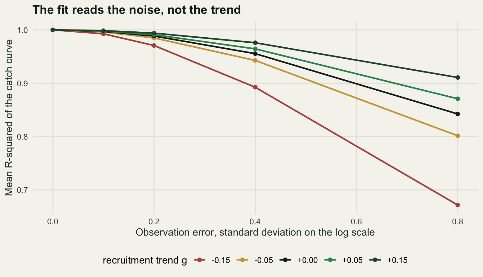

Figure 5: Mean R-squared of the catch curve against the level of observation error, one line per recruitment trend rate. The lines meet at one when there is no observation error, whatever the trend, and separate only as the noise grows.

The obvious next move is to stop looking at R-squared and look at the residuals. Four checks cost nothing: the Durbin-Watson statistic, the lag-one residual correlation, a runs test on the residual signs, and a quadratic term in age. Each is calibrated below on its own simulated null, so every size is 0.05 by construction and the rows are directly comparable.

set.seed(20260817)

n_rep_cc <- 4000; sig_cc <- 0.2
xx_cc <- cc_ages - mean(cc_ages); m_cc <- length(cc_ages)
X_q <- cbind(1, cc_ages, cc_ages^2); qr_q <- qr(X_q); h_q <- chol2inv(qr.R(qr_q))[3, 3]

diag_cc <- function(mu) {
  Y <- mu + matrix(rnorm(n_rep_cc * m_cc, 0, sig_cc), m_cc)
  out <- matrix(NA, n_rep_cc, 4, dimnames = list(NULL, c("dw", "r1", "runs", "quad")))
  for (i in seq_len(n_rep_cc)) {
    y <- Y[, i]
    e <- y - mean(y) - (sum(xx_cc * (y - mean(y))) / sum(xx_cc^2)) * xx_cc
    s <- sign(e); s[s == 0] <- 1
    bq <- qr.coef(qr_q, y); rq <- y - X_q %*% bq
    out[i, ] <- c(sum(diff(e)^2) / sum(e^2), sum(e[-1] * e[-m_cc]) / sum(e^2),
                  1 + sum(s[-1] != s[-m_cc]),
                  abs(bq[3]) / sqrt(sum(rq^2) / (m_cc - 3) * h_q))
  }
  out
}

null_cc <- diag_cc(log(caa_year(0)[cc_ages]))
cut_cc <- list(dw = quantile(null_cc[, "dw"], c(0.025, 0.975)),
               r1 = quantile(abs(null_cc[, "r1"]), 0.95),
               runs = quantile(null_cc[, "runs"], c(0.025, 0.975)),
               quad = quantile(null_cc[, "quad"], 0.95))

reject_cc <- function(s)
  c(`Durbin-Watson` = mean(s[, "dw"] < cut_cc$dw[1] | s[, "dw"] > cut_cc$dw[2]),
    `lag-1 residual r` = mean(abs(s[, "r1"]) > cut_cc$r1),
    `runs test` = mean(s[, "runs"] < cut_cc$runs[1] | s[, "runs"] > cut_cc$runs[2]),
    `quadratic in age` = mean(s[, "quad"] > cut_cc$quad))

cases_cc <- list(
  `no trend, the size` = log(caa_year(0)[cc_ages]),
  `trend g = -0.06` = log(caa_year(g_dec)[cc_ages]),
  `trend g = -0.15` = log(caa_year(-0.15)[cc_ages]),
  `trend g = +0.15` = log(caa_year(0.15)[cc_ages]),
  `recruitment doubled 9 years ago` = log((caa_year(0) * ifelse(ages < 9, 2, 1))[cc_ages]))

pow_cc <- t(vapply(cases_cc, function(mu) reject_cc(diag_cc(mu)), numeric(4)))
cc_pow_se <- sqrt(0.25 / n_rep_cc)
print(round(cbind(pow_cc, `MC SE at most` = cc_pow_se), 4))

                                Durbin-Watson lag-1 residual r runs test
no trend, the size                     0.0510           0.0535    0.0243
trend g = -0.06                        0.0490           0.0488    0.0187
trend g = -0.15                        0.0510           0.0478    0.0267
trend g = +0.15                        0.0538           0.0515    0.0213
recruitment doubled 9 years ago        0.3292           0.0585    0.1035
                                quadratic in age MC SE at most
no trend, the size                        0.0455        0.0079
trend g = -0.06                           0.0560        0.0079
trend g = -0.15                           0.0530        0.0079
trend g = +0.15                           0.0520        0.0079
recruitment doubled 9 years ago           0.5840        0.0079

cc_pow_size <- max(pow_cc[1, ]); cc_pow_max <- max(pow_cc[2:4, ])

cc_count <- function(g, n_fish, nrep = 2000) {
  p <- caa_year(g); p <- p / sum(p); zz <- r2 <- numeric(nrep)
  for (i in seq_len(nrep)) {
    y <- as.vector(rmultinom(1, n_fish, p))[cc_ages]; k <- y > 0
    xx <- cc_ages[k] - mean(cc_ages[k]); yy <- log(y[k]) - mean(log(y[k]))
    zz[i] <- -sum(xx * yy) / sum(xx^2)
    r2[i] <- (sum(xx * yy)^2 / sum(xx^2)) / sum(yy^2)
  }
  c(gap = mean(zz) - (m_base + f_cc + g), r2 = mean(r2))
}
cc_counts <- t(vapply(c(2000, 10000, 50000), function(n) {
  a <- cc_count(g_dec, n); b <- cc_count(0, n)
  c(fish_aged = n, gap_vs_Z_plus_g = unname(a["gap"]),
    r2_change_under_trend = unname(a["r2"] - b["r2"]))
}, numeric(3)))
print(signif(cc_counts, 3))

     fish_aged gap_vs_Z_plus_g r2_change_under_trend
[1,]      2000        5.87e-03               0.00130
[2,]     10000        1.83e-03               0.00547
[3,]     50000       -4.85e-05               0.00100

## one year class followed across years, in the same population trending at g_dec.
## It recruited once, so its own strength is one constant across all the ages it is met at.
coh_recr <- exp(-g_dec * (min(cc_ages) - 1))     # its recruitment, relative to the current year
coh_mu   <- log(coh_recr * caa_year(0)[cc_ages]) # its catch at age, same Z at every age
coh_cc <- coh_mu + matrix(rnorm(n_rep_cc * m_cc, 0, sig_cc), m_cc)
coh_cc <- coh_cc - rep(colMeans(coh_cc), each = m_cc)
bcc <- as.vector(crossprod(xx_cc, coh_cc)) / sum(xx_cc^2)
cc_cohort <- mean(-bcc); cc_cohort_se <- sd(bcc) / sqrt(n_rep_cc)
cc_cross <- unname(fit_cc(log(caa_year(g_dec)[cc_ages]))["Z"])
cat("\nrecruitment trending at", round(g_dec, 4),
    "\n  one year read across year classes:", round(cc_cross, 4),
    "\n  one year class followed across years:", round(cc_cohort, 4),
    "with a Monte Carlo standard error of", signif(cc_cohort_se, 2), "\n")

recruitment trending at -0.0619 
  one year read across year classes: 0.3376 
  one year class followed across years: 0.3993 with a Monte Carlo standard error of 0.00019 

Against a trend all four sit on their own size. The largest rejection rate across the three trend rows is 0.056, against 0.054 under the null and a Monte Carlo standard error of 0.0079. That is not weak power, it is none, and the reason is exact rather than statistical. Least squares residuals from a regression on age are unchanged when any straight line in age is added to the response, and a constant-rate recruitment trend adds exactly minus g times age. The residuals with a trend are the same random variables as the residuals without one, so any test computed from them has power equal to its size.

The last row of that table says the four checks are far from useless. Recruitment that doubled nine years ago biases the estimate too, but it is not log-linear, so it leaves curvature behind: the quadratic term picks it up 0.58 of the time and Durbin-Watson 0.33. Any recruitment history that bends the composition shows up in the residuals. The one that does not bend it is the one that maps cleanly onto the slope.

Two cautions belong with the numbers above. The error in the grid is additive on the log scale. Where the composition instead comes from ageing a finite sample of fish, a falling recruitment leaves more old fish in it, the counts in the tail get less noisy, and R-squared moves up rather than down: with 10000 fish aged the change is +0.0055. The same finite sample also leaves the slope above Z + g, by 0.0059 at 2000 fish, but that is a property of taking logs of small counts and of dropping the empty age classes, not of the estimator: at 50000 fish it is -0.00005.

The way out is not a better diagnostic. Follow one year class through successive years instead of reading one year across year classes. A cohort recruited once, so on the log scale its own strength is a single constant, the same at every age it is later met at, and it goes into the intercept where a regression on centred age removes it exactly. The last block puts that to work in the same population, with recruitment still falling 6 per cent a year. Read across year classes the line returns 0.3376, which is the trend added to the mortality rate. Read down the year class it returns 0.3993 with a Monte Carlo standard error of 0.00019, against the 0.3995 a noiseless fit gives: the true Z of 0.4 less the 0.000502 the still climbing selectivity costs, with the trend gone from it entirely. What that costs is age composition from more than one year. The tutorial on force of infection from age prevalence arrives at the same exit from a serological cross-section, where a rate that changed five years ago and a genuine age effect are not separable from one survey either.

The honest limit

Four things went into every reference point on this page: steepness, natural mortality, the shape of the recruitment curve, and the total mortality rate a catch curve returns. The measurements say that a thirty-year recruitment series with ordinary noise separates none of them. The likelihood interval for steepness covered 0.26 to 0.99; the two functional forms differed by 0.069 in AIC; natural mortality was never estimated at all, and the catch curve returned the mortality rate with the recruitment trend already added to it.

What the analysis cannot tell you is which value to use. It can only tell you what the choice costs. That makes reporting practice the actual issue. Fmsy = 0.16 is not a result; Fmsy = 0.16 given h = 0.7, M = 0.2 and a Beverton-Holt curve is a result, and a reader can then ask what happens at h = 0.5. A reference point quoted without its assumed steepness and natural mortality is a number quoted without its units.

Two further limits belong here. The equilibrium calculations assume the stock sits at a deterministic equilibrium, which it never does; recruitment variability alone means the realised yield at Fmsy is below MSY. And the whole exercise conditions on the life history being right, when growth, maturity and selectivity are themselves estimated from samples that the fishery selected.

Where to go next

Every number here started from a spawning biomass series, and in practice that series comes from an assessment fitted to an abundance index. The next tutorial in this cluster, on standardising catch per unit effort, deals with the index itself: what it takes to turn a commercial catch rate into something that tracks abundance, and how much of the trend survives the standardisation.

References

Ricker WE 1954 Journal of the Fisheries Research Board of Canada 11(5):559-623 (10.1139/f54-039)

Clark WG 1991 Canadian Journal of Fisheries and Aquatic Sciences 48(5):734-750 (10.1139/f91-088)

Myers RA, Bowen KG, Barrowman NJ 1999 Canadian Journal of Fisheries and Aquatic Sciences 56(12):2404-2419 (10.1139/f99-201)

Deroba JJ, Bence JR 2008 Fisheries Research 94(3):210-223 (10.1016/j.fishres.2008.01.003)

Mangel M, Brodziak J, DiNardo G 2010 Fish and Fisheries 11(1):89-104 (10.1111/j.1467-2979.2009.00345.x)

Related tutorials

• Surplus production models in R
• Standardising catch per unit effort
• Checking a stock assessment
• Fitting growth curves with nls