library(ggplot2)

te_pal <- list(forest = "#275139", green = "#2f8f63", sage = "#93a87f",
               clay = "#b5534e", gold = "#cda23f", line = "#dad9ca",
               ink = "#16241d", paper = "#f5f4ee")

theme_te <- function() {
  theme_minimal(base_size = 12) +
    theme(panel.grid.minor = element_blank(),
          panel.grid.major = element_line(colour = "#e7e6dc"),
          plot.background = element_rect(fill = "#f5f4ee", colour = NA),
          panel.background = element_rect(fill = "#f5f4ee", colour = NA),
          plot.title = element_text(face = "bold", colour = te_pal$ink),
          axis.title = element_text(colour = te_pal$ink))
}Standardising catch per unit effort
R
fisheries
stock assessment
GLM
ecology tutorial
ggplot2
Standardise fishery catch per unit effort in R with a GLM built by hand, then measure how hyperstability still hides a collapsing stock from the index.
Almost every stock assessment rests on one quiet assumption: that some index of abundance is proportional to biomass. The surplus production model in Surplus production models in R fits its trajectory to an index. The steepness estimate in Stock-recruitment and reference points depends on a biomass series that came from an index. In most fisheries that index is catch per unit effort from the commercial fleet, because it is the only long series anyone has. Take the proportionality as read in those two posts; this one examines it.
Two things break the proportionality, and they break it in different ways. The first is that the fleet changes. Vessels get better, effort moves to better ground, the season shifts, and the catch rate of the average trip changes without the stock changing at all. That problem has a standard answer: fit a model with year, vessel, area and season, and read the year effects. It works, and this post builds it by hand and measures how much it recovers.
The second is that catchability itself changes with abundance. When a stock thins out, fishers do not spread out with it; they go to the aggregations that remain, and the catch rate on those aggregations holds up. The index then falls more slowly than the stock. This one has no answer inside the data, and the measurement below is the point of the post: a standardised index is standardised for the fleet, not for the fish.
A fleet that changes underneath the index
The simulated fishery has twenty years of logbook records, two hundred and forty trips a year, twelve vessels, three areas of different density and two seasons. Six of the vessels are older and less efficient; six are newer. Over the series the newer vessels take a growing share of the trips, and effort also shifts towards the densest of the three areas, which is what a fleet with better plotters and better information does. True biomass declines steadily by seventy per cent.
Catch rate on a trip is the product of catchability, biomass, a vessel effect, an area effect, a season effect, an annual deviation in catchability shared by every trip in that year, and lognormal trip noise. That last shared deviation matters later: it is real year-to-year variation in how catchable the stock is, and no amount of data cleaning removes it.
set.seed(20260818)

n_year <- 20
n_trip <- 240
yrs <- 1:n_year

depl_end <- 0.30
biomass <- depl_end^((yrs - 1) / (n_year - 1))

n_ves <- 12
ves_eff <- c(rnorm(6, 0, 0.12), rnorm(6, 0.45, 0.12))
ves_new <- c(rep(FALSE, 6), rep(TRUE, 6))

area_eff <- log(c(0.6, 1.0, 1.8))
seas_eff <- log(c(0.85, 1.25))

p_new <- seq(0.15, 0.80, length.out = n_year)
w_area <- cbind(seq(0.45, 0.15, length.out = n_year),
                seq(0.35, 0.30, length.out = n_year),
                seq(0.20, 0.55, length.out = n_year))
w_area <- w_area / rowSums(w_area)

proc_err <- rnorm(n_year, 0, 0.10)
obs_sd <- 0.35
q0 <- 0.02

make_trips <- function(bio, hyper = 1) {
  out <- vector("list", n_year)
  for (i in seq_len(n_year)) {
    isnew <- runif(n_trip) < p_new[i]
    vid <- ifelse(isnew, sample(7:12, n_trip, TRUE), sample(1:6, n_trip, TRUE))
    aid <- sample(1:3, n_trip, TRUE, prob = w_area[i, ])
    sid <- sample(1:2, n_trip, TRUE)
    mu <- log(q0) + hyper * log(bio[i]) + proc_err[i] +
      ves_eff[vid] + area_eff[aid] + seas_eff[sid]
    out[[i]] <- data.frame(yr = i, ves = vid, ar = aid, se = sid,
                           cpue = exp(mu + rnorm(n_trip, 0, obs_sd)))
  }
  do.call(rbind, out)
}

trips <- make_trips(biomass)

cat("years:", n_year, " trips per year:", n_trip, " records:", nrow(trips), "\n")
years: 20 trips per year: 240 records: 4800 cat("vessels:", n_ves, " areas: 3 seasons: 2 trip noise sd:", obs_sd, "\n")vessels: 12 areas: 3 seasons: 2 trip noise sd: 0.35 cat("process error sd: 0.1 true decline:",
round(1 - biomass[n_year] / biomass[1], 4), "\n")process error sd: 0.1 true decline: 0.7 cat("newer-vessel share of trips, year 1 and year 20:",
round(p_new[1], 2), round(p_new[n_year], 2), "\n")newer-vessel share of trips, year 1 and year 20: 0.15 0.8 cat("densest-area share of trips, year 1 and year 20:",
round(w_area[1, 3], 2), round(w_area[n_year, 3], 2), "\n")densest-area share of trips, year 1 and year 20: 0.2 0.55 cat("mean efficiency ratio, newer over older vessels:",
round(exp(mean(ves_eff[ves_new]) - mean(ves_eff[!ves_new])), 3), "\n")mean efficiency ratio, newer over older vessels: 1.688 The nominal index is what a spreadsheet gives you: the mean catch rate of all trips in a year. Compare it to the truth on the log scale, since both are only defined up to a constant, and normalise each series to its own geometric mean.
norm1 <- function(x) x / exp(mean(log(x)))
dec_trend <- function(idx) 1 - exp(unname(coef(lm(log(idx) ~ yrs))[2]) * (n_year - 1))

true_i <- norm1(biomass)
nom_i <- norm1(as.numeric(tapply(trips$cpue, trips$yr, mean)))

cat("true decline over the series:", round(dec_trend(true_i), 4), "\n")
true decline over the series: 0.7 cat("nominal CPUE decline:", round(dec_trend(nom_i), 4), "\n")nominal CPUE decline: 0.4193 cat("gap in decline:", round(dec_trend(true_i) - dec_trend(nom_i), 4), "\n")gap in decline: 0.2807 cat("slope of log nominal on log true:",
round(coef(lm(log(nom_i) ~ log(true_i)))[2], 4), "\n")slope of log nominal on log true: 0.4515 The stock lost 70 per cent of its biomass and the nominal index reports a loss of 41.93 per cent, a gap of 28.07 percentage points. The slope of log nominal on log true is 0.4515, which is worth staring at: the fleet effect alone, with catchability perfectly constant, has produced a fitted relationship that looks exactly like hyperstability with an exponent well below one. Two changes that any fishery manager would call progress, better vessels and better targeting, have eaten a large part of the signal.
d_idx <- data.frame(yr = rep(yrs, 2),
                    value = c(true_i, nom_i),
                    series = rep(c("True biomass", "Nominal CPUE"), each = n_year),
                    panel = "Index (geometric mean 1)")
d_mix <- data.frame(yr = rep(yrs, 2),
                    value = c(p_new, w_area[, 3]),
                    series = rep(c("Newer vessels", "Densest area"), each = n_year),
                    panel = "Share of trips")
d_both <- rbind(d_idx, d_mix)

p1 <- ggplot(d_both, aes(yr, value, colour = series)) +
  geom_line(linewidth = 1.1) +
  facet_wrap(~ panel, ncol = 1, scales = "free_y") +
  scale_colour_manual(values = c("True biomass" = te_pal$forest,
                                 "Nominal CPUE" = te_pal$clay,
                                 "Newer vessels" = te_pal$green,
                                 "Densest area" = te_pal$gold)) +
  labs(title = "The fleet changes, the index follows the fleet",
       x = "Year", y = NULL, colour = NULL) +
  theme_te() + theme(legend.position = "bottom")
p1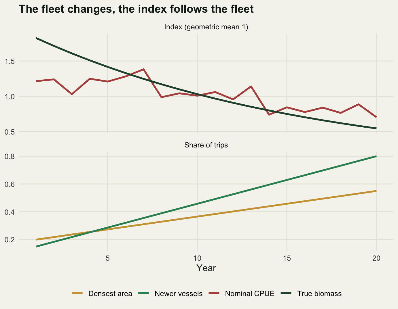
Standardising by hand, and the trap in the prediction step
The standard fix is a linear model of log catch rate on year, vessel, area and season, with year as a factor so that no shape is imposed on the trend. The year effects are then the index. The part people get wrong is not the fit; it is what you do with the fit afterwards.
The right operation is a least-squares mean: predict the model at a fixed reference set of vessels, areas and seasons, holding that set the same in every year, and let only the year term move. Below, the reference set is every combination of the twelve vessels, three areas and two seasons, equally weighted.
trips$fy <- factor(trips$yr); trips$fv <- factor(trips$ves)
trips$fa <- factor(trips$ar); trips$fs <- factor(trips$se)

fit <- lm(log(cpue) ~ fy + fv + fa + fs, data = trips)

ref <- expand.grid(fy = factor(1, levels = levels(trips$fy)),
                   fv = factor(1:n_ves, levels = levels(trips$fv)),
                   fa = factor(1:3, levels = levels(trips$fa)),
                   fs = factor(1:2, levels = levels(trips$fs)))

ls_index <- function(model, dat_ref) {
  vals <- sapply(levels(trips$fy), function(y) {
    g <- dat_ref
    g$fy <- factor(y, levels = levels(trips$fy))
    mean(predict(model, g))
  })
  norm1(exp(as.numeric(vals)))
}

std_i <- ls_index(fit, ref)
obs_i <- norm1(exp(as.numeric(tapply(predict(fit), trips$yr, mean))))

cat("reference rows:", nrow(ref), "\n")
reference rows: 72 cat("standardised decline (fixed reference set):", round(dec_trend(std_i), 4), "\n")standardised decline (fixed reference set): 0.7049 cat("standardised decline (observed mix):", round(dec_trend(obs_i), 4), "\n")standardised decline (observed mix): 0.4131 cat("slope of log standardised on log true:",
round(coef(lm(log(std_i) ~ log(true_i)))[2], 4), "\n")slope of log standardised on log true: 1.0136 rmse <- function(a, b) sqrt(mean((log(a) - log(b))^2))
cat("log-scale RMSE, nominal:", round(rmse(nom_i, true_i), 4), "\n")log-scale RMSE, nominal: 0.2278 cat("log-scale RMSE, standardised:", round(rmse(std_i, true_i), 4), "\n")log-scale RMSE, standardised: 0.093 cat("log-scale RMSE, observed mix:", round(rmse(obs_i, true_i), 4), "\n")log-scale RMSE, observed mix: 0.2282 cat("improvement factor:", round(rmse(nom_i, true_i) / rmse(std_i, true_i), 2), "\n")improvement factor: 2.45 The standardised index reports a decline of 70.49 per cent against a true 70 per cent, and the slope on the truth is 1.0136. The log-scale error falls from 0.2278 to 0.093, an improvement of 2.45 times. That residual 0.093 is not a failure of the method: it is close to the annual process error of 0.1 that went into the simulation. The index is tracking the realised catchability of each year, which is what it is supposed to do, and no covariate can remove variation that was never recorded.
The trap is the second line. Predicting from the same fitted model, but at the covariate mix that was actually observed in each year, and averaging those predictions, gives 41.31 per cent: the nominal answer, to within noise. The model was correct, the coefficients were correct, and the index is still wrong, because averaging over a mix that drifts puts the drift straight back in. This is easy to do by accident, because predict(fit) with no newdata is the shortest line of code in the script.
ref2 <- trips[trips$yr == 1, c("fy", "fv", "fa", "fs")]
std2 <- ls_index(fit, ref2)
cat("largest absolute difference between two reference sets:",
    signif(max(abs(std_i - std2)), 3), "\n")
largest absolute difference between two reference sets: 8.88e-16 Which fixed reference set you choose does not matter here, and it is worth knowing why. With a purely additive model the other terms contribute the same constant to every year, so they cancel in the year-to-year ratios: swapping the balanced grid for the year 1 fleet moves the index by about 1e-15. The reference set starts to matter as soon as the model has a year interaction, for instance year by area when the areas are fished in different proportions; then you are choosing what “the fishery” means, and the choice is a judgement, not a default.
lev_std <- c("True biomass", "Standardised (fixed set)",
             "Nominal", "Standardised (observed mix)")
d_std <- data.frame(
  yr = rep(yrs, 4),
  value = c(true_i, nom_i, std_i, obs_i),
  series = factor(rep(c("True biomass", "Nominal", "Standardised (fixed set)",
                        "Standardised (observed mix)"), each = n_year), levels = lev_std))

p2 <- ggplot(d_std, aes(yr, value, colour = series, linetype = series)) +
  geom_line(linewidth = 1.1) +
  scale_colour_manual(values = c("True biomass" = te_pal$forest,
                                 "Standardised (fixed set)" = te_pal$green,
                                 "Nominal" = te_pal$clay,
                                 "Standardised (observed mix)" = te_pal$gold)) +
  scale_linetype_manual(values = c("True biomass" = "solid",
                                   "Standardised (fixed set)" = "22",
                                   "Nominal" = "solid",
                                   "Standardised (observed mix)" = "22")) +
  labs(title = "Standardisation works, if you predict at a fixed reference set",
       x = "Year", y = "Index (geometric mean 1)",
       colour = NULL, linetype = NULL) +
  theme_te() + theme(legend.position = "bottom")
p2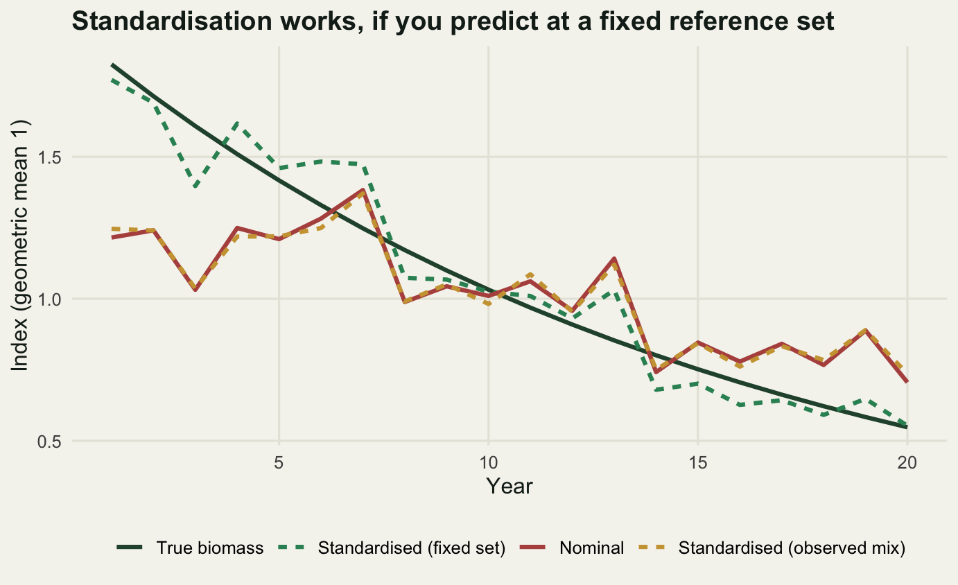
Hyperstability: the part the GLM cannot reach
Now change one thing in the generating process. Instead of catch rate proportional to biomass, make it proportional to biomass raised to a power below one, so that catchability rises as the stock falls. The mechanism is not mysterious. Fish that school or aggregate to spawn keep their local density as their numbers drop, the aggregations just become fewer, and a fleet that knows where they are keeps filling its holds. Everything else stays as it was: same fleet drift, same vessels, same standardisation.
The stock now falls by 85 per cent, which in most jurisdictions would be a collapse.
set.seed(4471)
depl2 <- 0.15
bio2 <- depl2^((yrs - 1) / (n_year - 1))
b_exp <- c(1.0, 0.8, 0.6, 0.4)

hyp <- data.frame()
store <- list()
for (b in b_exp) {
  tr <- make_trips(bio2, hyper = b)
  tr$fy <- factor(tr$yr); tr$fv <- factor(tr$ves)
  tr$fa <- factor(tr$ar); tr$fs <- factor(tr$se)
  ft <- lm(log(cpue) ~ fy + fv + fa + fs, data = tr)
  vals <- sapply(levels(tr$fy), function(y) {
    g <- ref
    g$fy <- factor(y, levels = levels(tr$fy))
    mean(predict(ft, g))
  })
  si <- norm1(exp(as.numeric(vals)))
  store[[as.character(b)]] <- si
  hyp <- rbind(hyp, data.frame(exponent = b,
                               index_decline = dec_trend(si),
                               expected = 1 - depl2^b,
                               true_B_at_index_0.6 = 0.6^(1 / b),
                               true_B_at_index_0.8 = 0.8^(1 / b)))
}

cat("true decline:", round(dec_trend(norm1(bio2)), 4), "\n")
true decline: 0.85 print(round(hyp, 4)) exponent index_decline expected true_B_at_index_0.6 true_B_at_index_0.8
1 1.0 0.8531 0.8500 0.6000 0.8000
2 0.8 0.7818 0.7808 0.5281 0.7566
3 0.6 0.6846 0.6796 0.4268 0.6894
4 0.4 0.5342 0.5318 0.2789 0.5724Read the second column against the first. With the exponent at one the standardised index gets the collapse right: 85.31 per cent against a true 85 per cent. At 0.8 it reports 78.18 per cent, at 0.6 it reports 68.46 per cent, and at 0.4 it reports 53.42 per cent. The fleet standardisation is working perfectly in all four cases. The year effects are unbiased estimates of the thing the catch rate is proportional to, and the catch rate is proportional to the wrong thing.
The last two columns are what a manager would care about. Take an index reading of 0.6 of the unfished level, a common trigger for concern. At an exponent of 0.6 the stock is actually at 0.4268 of unfished when the index first reads 0.6, and at an exponent of 0.4 it is at 0.2789. Take the softer reading of 0.8, the kind of number that gets a fishery described as lightly fished: at an exponent of 0.4 the stock is at 0.5724 of unfished, more than two fifths gone, while the index says it has lost a fifth.
Nothing in the logbook data distinguishes these four fisheries. They have the same vessels, the same areas, the same seasons, and the same well-behaved residuals. You can add every covariate you own and the exponent will not move, because the exponent is a property of how fish and fishers are distributed in space, not a property of the sampling design that the model knows about.
lev_exp <- as.character(b_exp)
d_hyp <- do.call(rbind, lapply(lev_exp, function(k) {
  data.frame(depletion = bio2 / bio2[1],
             idx = store[[k]] / store[[k]][1],
             exponent = factor(k, levels = lev_exp))
}))
d_mark <- data.frame(depletion = hyp$true_B_at_index_0.6,
                     idx = rep(0.6, nrow(hyp)),
                     exponent = factor(lev_exp, levels = lev_exp))

d_one <- data.frame(depletion = c(min(d_hyp$depletion), 1),
                    idx = c(min(d_hyp$depletion), 1))

p3 <- ggplot(d_hyp, aes(depletion, idx, colour = exponent)) +
  geom_line(data = d_one, aes(depletion, idx), inherit.aes = FALSE,
            colour = te_pal$sage, linewidth = 0.9, linetype = "22") +
  geom_hline(yintercept = 0.6, colour = te_pal$line, linewidth = 0.9) +
  geom_line(linewidth = 1.1) +
  geom_point(data = d_mark, size = 2.6) +
  scale_colour_manual(values = c("1" = te_pal$forest, "0.8" = te_pal$green,
                                 "0.6" = te_pal$gold, "0.4" = te_pal$clay)) +
  scale_x_reverse() +
  annotate("text", x = 0.30, y = 0.14, label = "one to one",
           colour = te_pal$sage, size = 3.4, hjust = 1) +
  labs(title = "The index stays high while the stock falls",
       x = "True biomass as a proportion of unfished (axis reversed)",
       y = "Standardised index relative to year 1",
       colour = "Exponent") +
  theme_te()
p3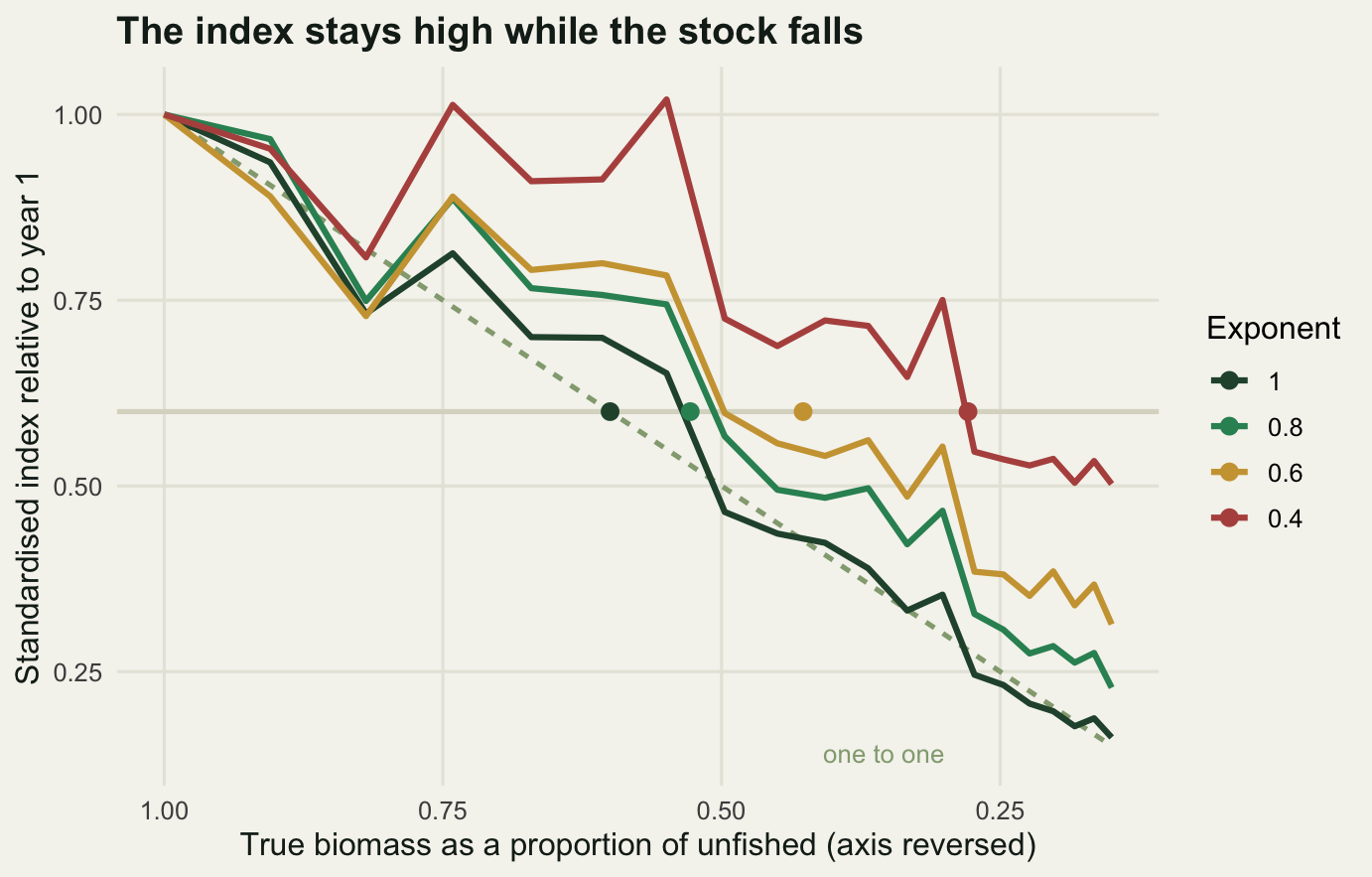
What an independent survey buys
The only measurement that can settle this comes from outside the fishery: a survey that fixes its own stations, uses its own gear, and does not chase aggregations. Surveys are small, so the question is how small a survey still helps. Here the survey is unbiased with respect to biomass and has a per-station log-scale noise of 1.4, which is a patchy stock; averaging over stations divides that noise by the square root of the number of stations.
The CPUE index is the hyperstable one with an exponent of 0.6, which reported 68.46 per cent against a true 85 per cent. Each index gives a decline estimate from a log-linear trend across the twenty years. The obvious way to use both is inverse-variance weighting of the two slopes, which is what a joint likelihood does if you give each index its own observation error and nothing else.
set.seed(991)
cp_idx <- store[["0.6"]]
sig_c <- summary(lm(log(cp_idx) ~ yrs))$sigma
sig_station <- 1.4
n_rep <- 500
n_st <- c(20, 60, 196, 800)

sl_c <- unname(coef(lm(log(cp_idx) ~ yrs))[2])
dec_c <- 1 - exp(sl_c * (n_year - 1))
tab <- data.frame()
for (nn in n_st) {
  ss <- sig_station / sqrt(nn)
  w_sv <- (1 / ss^2) / (1 / ss^2 + 1 / sig_c^2)
  d_sv <- numeric(n_rep); d_cb <- numeric(n_rep); excl <- logical(n_rep)
  for (r in seq_len(n_rep)) {
    sv <- norm1(bio2 * exp(rnorm(n_year, 0, ss)))
    fs2 <- lm(log(sv) ~ yrs)
    sl_s <- unname(coef(fs2)[2]); se_s <- summary(fs2)$coefficients[2, 2]
    d_sv[r] <- 1 - exp(sl_s * (n_year - 1))
    d_cb[r] <- 1 - exp((w_sv * sl_s + (1 - w_sv) * sl_c) * (n_year - 1))
    lo <- 1 - exp((sl_s + 1.96 * se_s) * (n_year - 1))
    hi <- 1 - exp((sl_s - 1.96 * se_s) * (n_year - 1))
    excl[r] <- dec_c < lo || dec_c > hi
  }
  tab <- rbind(tab, data.frame(stations = nn, survey_weight = w_sv,
                               survey_dec = mean(d_sv), survey_sd = sd(d_sv),
                               combined_dec = mean(d_cb),
                               p_reject_cpue = mean(excl)))
}

cat("replicates per station count:", n_rep, "\n")
replicates per station count: 500 cat("per-station survey noise sd:", sig_station, "\n")per-station survey noise sd: 1.4 cat("CPUE residual sd about its trend:", round(sig_c, 4), "\n")CPUE residual sd about its trend: 0.097 cat("stations needed to match CPUE precision:",
round((sig_station / sig_c)^2, 1), "\n")stations needed to match CPUE precision: 208.4 cat("true decline:", round(dec_trend(norm1(bio2)), 4),
" CPUE-only decline:", round(dec_c, 4), "\n")true decline: 0.85 CPUE-only decline: 0.6846 print(round(tab, 4)) stations survey_weight survey_dec survey_sd combined_dec p_reject_cpue
1 20 0.0875 0.8449 0.0331 0.7041 0.880
2 60 0.2235 0.8483 0.0190 0.7325 0.998
3 196 0.4846 0.8501 0.0106 0.7802 1.000
4 800 0.7933 0.8500 0.0054 0.8251 1.000The survey alone lands close to the truth at every size: 0.8449 at twenty stations against a true 0.85, and 0.8500 at eight hundred. What changes most with size is the spread, from 0.0331 at twenty stations to 0.0054 at eight hundred. The centre moves a little as well, because the decline is a concave function of the fitted slope, so the wider slope scatter of a small survey pulls the mean decline down by a few thousandths.
Two results here were not what I expected, and both survive rerunning. The first is how little survey you need to contradict the assessment. At twenty stations, a survey small enough to run from one boat in a fortnight, the 95 per cent interval on the survey’s own decline estimate excludes the CPUE answer in 88 per cent of replicates, and at sixty stations in 99.8 per cent. The bias from hyperstability is far larger than the sampling error of even a poor survey, so the survey does not need to be precise to be decisive.
The second is how badly inverse-variance weighting handles the pair. To match the CPUE index for precision the survey needs 208.4 stations, because the CPUE index is very precise: its residual scatter about the trend is only 0.097, essentially the process error, since it averages thousands of trips. Below that the survey gets minority weight, and the combined estimate is pulled towards the biased index: 0.7041 at twenty stations against a CPUE-only 0.6846 and a true 0.85. Even at 196 stations, with the weight at 0.4846, the combination reports 0.7802. The weighting is doing exactly what it was asked to do, which is to favour the more precise index, and precision is not the problem. Combining an unbiased index with a biased one by variance alone buys you a more precise wrong answer.
The practical reading is that the survey is a check, not an ingredient. If the survey and the CPUE index disagree by more than the survey’s own uncertainty, the honest conclusion is that the CPUE index has a catchability problem, and the right response is to downweight it by hand or fit the exponent as a parameter with the survey identifying it, not to average the two.
d_sur <- rbind(
  data.frame(stations = tab$stations, est = tab$survey_dec,
             lo = tab$survey_dec - 1.96 * tab$survey_sd,
             hi = tab$survey_dec + 1.96 * tab$survey_sd,
             method = "Survey alone"),
  data.frame(stations = tab$stations, est = tab$combined_dec,
             lo = tab$combined_dec, hi = tab$combined_dec,
             method = "Inverse-variance combination"))

p4 <- ggplot(d_sur, aes(factor(stations), est, colour = method)) +
  geom_hline(yintercept = dec_trend(norm1(bio2)), colour = te_pal$forest,
             linewidth = 0.8) +
  geom_hline(yintercept = dec_c, colour = te_pal$clay, linewidth = 0.8,
             linetype = "22") +
  geom_pointrange(aes(ymin = lo, ymax = hi), size = 0.6,
                  position = position_dodge(width = 0.35)) +
  scale_colour_manual(values = c("Survey alone" = te_pal$green,
                                 "Inverse-variance combination" = te_pal$gold)) +
  annotate("text", x = 0.6, y = dec_trend(norm1(bio2)) + 0.012,
           label = "truth", colour = te_pal$forest, size = 3.4, hjust = 0) +
  annotate("text", x = 0.6, y = dec_c + 0.012, label = "CPUE alone",
           colour = te_pal$clay, size = 3.4, hjust = 0) +
  coord_cartesian(ylim = c(0.65, 0.93)) +
  labs(title = "A small survey is decisive; averaging it in is not",
       x = "Survey stations", y = "Estimated decline over the series",
       colour = NULL) +
  theme_te() + theme(legend.position = "bottom")
p4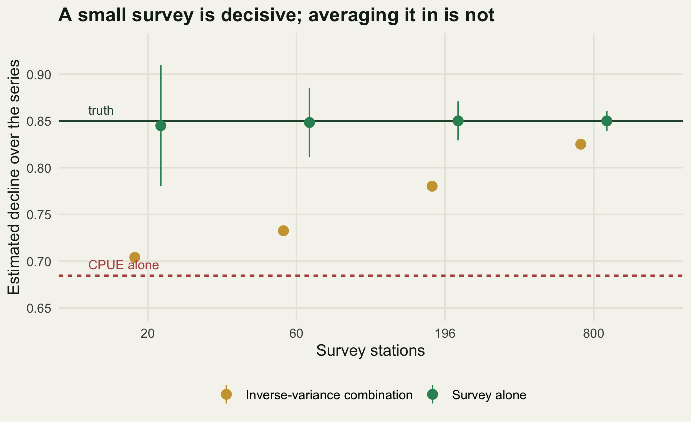
Zeros and the error structure
One more way to build a trend that is not there. Suppose the fraction of trips that catch nothing rises as the stock falls, which it does, and suppose the analyst drops the zeros and fits a lognormal to the positive catches only. Total catch rate is still exactly proportional to biomass here, with no hyperstability at all; the only change is that the proportion of positive trips falls from 0.9 to 0.432 across the series.
set.seed(707)
p_pos <- 0.35 + 0.55 * bio2
pos_only <- numeric(n_year)
delta_i <- numeric(n_year)
for (i in seq_len(n_year)) {
  isp <- runif(n_trip) < p_pos[i]
  mu <- log(q0 * bio2[i] / p_pos[i])
  y <- ifelse(isp, exp(rnorm(n_trip, mu - 0.5 * obs_sd^2, obs_sd)), 0)
  pos_only[i] <- mean(y[y > 0])
  delta_i[i] <- mean(y > 0) * mean(y[y > 0])
}
pos_only <- norm1(pos_only); delta_i <- norm1(delta_i)

cat("proportion positive, year 1 and year 20:",
    round(p_pos[1], 3), round(p_pos[n_year], 3), "\n")
proportion positive, year 1 and year 20: 0.9 0.432 cat("true decline:", round(dec_trend(norm1(bio2)), 4), "\n")true decline: 0.85 cat("positives-only index decline:", round(dec_trend(pos_only), 4), "\n")positives-only index decline: 0.6945 cat("delta index decline:", round(dec_trend(delta_i), 4), "\n")delta index decline: 0.8447 cat("induced bias:", round(dec_trend(norm1(bio2)) - dec_trend(pos_only), 4), "\n")induced bias: 0.1555 Dropping the zeros turns an 85 per cent decline into a 69.45 per cent decline, a bias of 15.55 percentage points that looks identical to hyperstability and has nothing to do with fish behaviour. The delta approach, which models the probability of a positive trip and the mean of the positives separately and multiplies them, gets back to 84.47 per cent. A Tweedie likelihood does the same job in one model rather than two, and if the zeros in your data are structural rather than an artefact of reporting that is usually the cleaner route: Tweedie regression for biomass data works through the error structure and the choice of the power parameter, which is not this post’s subject.
What standardisation cannot tell you
Standardisation removes the variation you thought to record. That sentence is the whole limit. The GLM above corrected the vessel and area drift perfectly because vessel identity and area were columns in the logbook. Everything that was not a column stayed in the index and came out looking like abundance.
The list of things that are usually not columns is long and unhappy. Targeting is the first: a vessel that switched from one species to another has a changed catch rate for the first species and the logbook records only that it fished. Gear creep is the second: a vessel keeps its name and its length while its electronics, its line, its net and its skipper’s knowledge all improve, so the vessel effect that the model assumes is constant is a slow trend. Reporting changes are the third, and they are the worst, because a new logbook form or a new enforcement regime can move recorded effort by a large factor in one year. Regulation-driven shifts are the fourth: a closed area, a trip limit or a seasonal restriction moves the fleet in ways that correlate with abundance by design. Each one of these enters the index as a change in catch rate, and a change in catch rate is what the model is reading as a change in abundance.
The hyperstability result is the sharp version of the same point, because there the missing variable is not even in principle recordable from the fishery. The exponent is a statement about how fish density responds to fish abundance, and a fleet that is good at finding fish is exactly the instrument least able to measure it.
So the only external check is an independent survey, and the survey has to be independent in the part that matters: fixed stations, fixed gear, no response to where the fish are this year. When the assessment and the survey disagree, the assessment is not automatically right. The assessment usually has more data, a longer series and a tighter fit, and none of that is evidence about catchability. The survey is the one series whose relationship to biomass you designed rather than inherited, and a conflict is information about the assessment, not noise to be smoothed away.
Where to go next
The natural next step is to stop trusting the fit and start testing it. Take the standardised index into an assessment, then check whether the assessment can be broken: retrospective patterns as new years are added, conflict between the index and the catch composition, and the behaviour of the residuals when the index is systematically wrong in the way this post simulated. Checking a stock assessment works through those diagnostics on a fitted model, and the hyperstable index built here is a good thing to feed it.
References
Maunder MN, Punt AE 2004 Fisheries Research 70(2-3):141-159 (10.1016/j.fishres.2004.08.002)
Harley SJ, Myers RA, Dunn A 2001 Canadian Journal of Fisheries and Aquatic Sciences 58(9):1760-1772 (10.1139/f01-112)
Erisman BE, Allen LG, Claisse JT, Pondella DJ, Miller EF, Murray JH 2011 Canadian Journal of Fisheries and Aquatic Sciences 68(10):1705-1716 (10.1139/f2011-090)
Campbell RA 2004 Fisheries Research 70(2-3):209-227 (10.1016/j.fishres.2004.08.026)
Walters C 2003 Canadian Journal of Fisheries and Aquatic Sciences 60(12):1433-1436 (10.1139/f03-152)
Hilborn R, Walters CJ 1992 Quantitative Fisheries Stock Assessment. Chapman and Hall, ISBN 978-0-412-02271-5