Fat-tailed dispersal kernels

Thin-tailed and fat-tailed dispersal kernels fit the same seed-trap data yet disagree by orders of magnitude on long-distance dispersal. A comparison in R.

Most of a dispersal kernel is uninteresting. Seeds pile up near the source, and any sensible density captures that. The part that matters for how a population moves is the far tail: the rare seed that travels ten or a hundred times the median distance. Those events set how fast a range expands, how far genes flow between patches, and how quickly an invader colonises new ground. When trees were found to have tracked postglacial warming faster than a thin-tailed kernel could explain (Reid’s paradox), the resolution was that the tail is fatter than a Gaussian, so a few long jumps do the work of many short ones.

So the tail is the whole point, and it is exactly the part the data pins down worst. This tutorial makes that concrete: fit several kernel families to the same seed rain, and watch them agree on the bulk while disagreeing by orders of magnitude on the tail.

Thin tails and fat tails

Four location kernels span the range from thin to fat. Written as distance densities k_D(r) = 2\pi r\,f(r) (the form you fit to trap distances, see the previous tutorial):

• Gaussian, k_D(r) \propto r\,e^{-(r/a)^2}. The tail falls like e^{-r^2}: the thinnest of the four, essentially no long-distance dispersal.
• Exponential, k_D(r) \propto r\,e^{-r/a}. Tail falls like e^{-r}, still thin.
• Exponential-power, k_D(r) \propto r\,e^{-(r/a)^c}. With shape c < 1 the tail is a stretched exponential, fatter than the exponential but not heavy.
• 2Dt (a two-dimensional Student-t), k_D(r) \propto r\,(1 + r^2/a^2)^{-(p+1)}. The tail falls like a power law, r^{-(2p+1)}. This is a heavy tail: it decays polynomially, not exponentially, so very long jumps stay possible.

kd_gauss <- function(r, a)    (2 * r / a^2) * exp(-(r / a)^2)
kd_exp   <- function(r, a)    (r / a^2) * exp(-r / a)
kd_ep    <- function(r, a, c) (c * r / (a^2 * gamma(2 / c))) * exp(-(r / a)^c)
kd_2dt   <- function(r, a, p) (2 * p * r / a^2) * (1 + r^2 / a^2)^(-(p + 1))
# survival functions P(r > R)
S_gauss <- function(R, a)    exp(-(R / a)^2)
S_exp   <- function(R, a)    exp(-R / a) * (1 + R / a)
S_ep    <- function(R, a, c) pgamma((R / a)^c, shape = 2 / c, lower.tail = FALSE)
S_2dt   <- function(R, a, p) (1 + R^2 / a^2)^(-p)

Now simulate a seed rain from a fat-tailed truth (a 2Dt with a power-law tail) and fit all four families by maximum likelihood.

set.seed(202)
a_true <- 25; p_true <- 1.5; n <- 600
r <- a_true * sqrt((1 - runif(n))^(-1 / p_true) - 1)   # 2Dt distances, tail ~ r^-4

fit1 <- function(nll, lo, hi) exp(optimize(nll, c(lo, hi))$minimum)
a_g <- fit1(function(la) -sum(log(kd_gauss(r, exp(la)))), -5, 12)
a_e <- fit1(function(la) -sum(log(kd_exp(r, exp(la)))), -5, 12)
op  <- optim(c(log(median(r)), 0), function(v) -sum(log(kd_ep(r, exp(v[1]), exp(v[2])))), method = "BFGS")
a_p <- exp(op$par[1]); c_p <- exp(op$par[2])
ot  <- optim(c(log(median(r)), 0), function(v) -sum(log(kd_2dt(r, exp(v[1]), exp(v[2])))), method = "BFGS")
a_t <- exp(ot$par[1]); p_t <- exp(ot$par[2])

ll <- function(f) sum(log(f))
aic <- c(gauss = 2 * 1 - 2 * ll(kd_gauss(r, a_g)),
         exp   = 2 * 1 - 2 * ll(kd_exp(r, a_e)),
         `exp-power` = 2 * 2 - 2 * ll(kd_ep(r, a_p, c_p)),
         `2Dt` = 2 * 2 - 2 * ll(kd_2dt(r, a_t, p_t)))

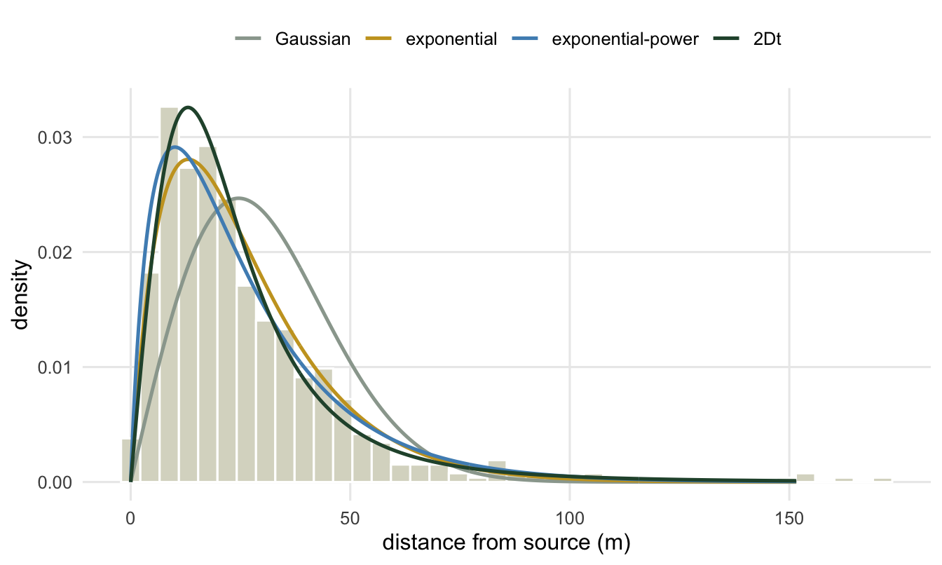
The heavy-tailed families win clearly. The 2Dt recovers the truth (fitted p = 1.45, scale 25.8 m, against p = 1.5, scale 25 m). Its AIC is 5011, against 5020 for the exponential-power, 5036 for the exponential, and 5345 for the Gaussian. On this dataset you can see the fat tail: the observed 99th percentile is 127 m, far past anything a Gaussian with this bulk would allow.

Figure 1: The observed distances against the four fitted densities, over the range the data actually cover. The heavy-tailed 2Dt and exponential-power track the histogram into the tail; the Gaussian and exponential run short.

Where they part company

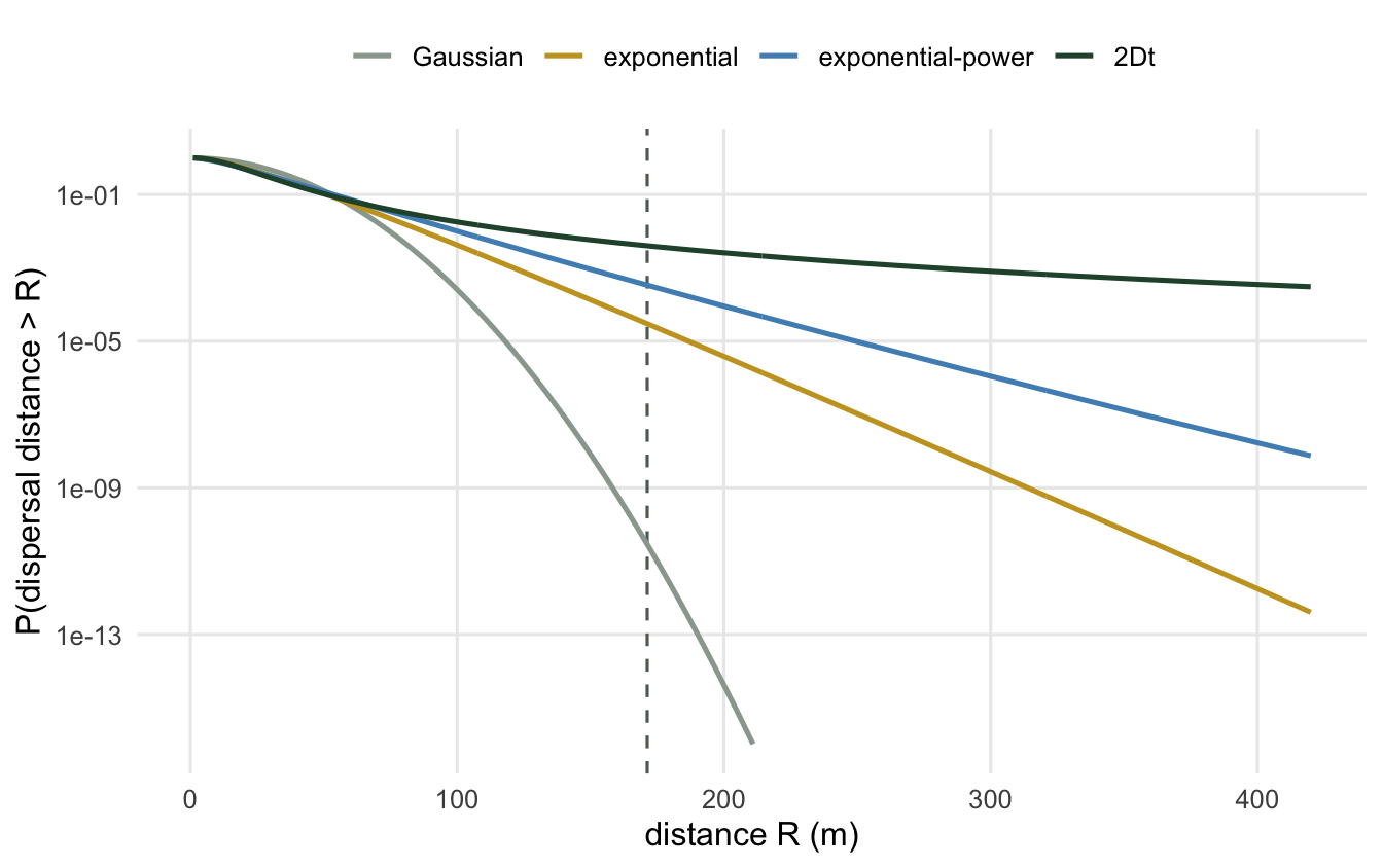
The bulk fit hides the disagreement, because the disagreement is in the tail, past the data. Compute the probability of a seed travelling further than a fixed distance under each fitted kernel.

tailP <- function(R) c(
  Gaussian = S_gauss(R, a_g), exponential = S_exp(R, a_e),
  `exp-power` = S_ep(R, a_p, c_p), `2Dt` = S_2dt(R, a_t, p_t))
p100 <- tailP(100); p200 <- tailP(200); p400 <- tailP(400)
ratio200 <- p200[["2Dt"]] / p200[["Gaussian"]]
max_obs <- max(r)

At 100 m, just past the observed range, the families are already spreading: the 2Dt puts 1.8 seeds in a hundred beyond that distance, the Gaussian only 0.0255. At 200 m, well past the furthest observed seed (171 m), the gap is a chasm: the 2Dt gives 2.6e-03, the exponential-power 9.0e-05, the exponential 3.9e-06, and the Gaussian 4.2e-15. The 2Dt and the Gaussian differ by a factor of 6e+11 at that one distance. At 400 m the Gaussian gives 3e-58, a number so small it means “never”, while the 2Dt still gives 4e-04, roughly one seed in three thousand.

Figure 2: The survival probability P(distance > R) under each fitted kernel, on a logarithmic scale. The four curves are close within the data (dashed line marks the furthest observed seed) and fan out by orders of magnitude beyond it. The far tail is pure extrapolation.

The uncomfortable part

Two lessons sit on top of each other here. The first is that the kernel family is not a cosmetic choice: it is the long-distance-dispersal prediction. Fit a Gaussian and you have decided, before seeing any far seed, that long jumps do not happen. Fit a 2Dt and you have allowed them. The bulk of the data does not decide this for you, because the bulk is the same either way.

The second is quieter. Even the 2Dt, which here recovers the truth, is extrapolating past the last observed seed at 171 m. Its estimate that one seed in three thousand reaches 400 m rests on the shape of a power law fitted mostly to seeds within 60 m. When the data do contain a fat tail, as here, you can at least tell a heavy family from a thin one. When they do not, which is the usual case with traps that only reach a short way, the families are indistinguishable in the bulk and the tail is a guess dressed as an estimate. The next tutorial follows the single quantity most exposed to this: the mean dispersal distance, which averages over the whole tail and can be infinite.

References

Clark JS 1998. American Naturalist 152(2):204-224 (10.1086/286162).

Clark JS, Silman M, Kern R, Macklin E, HilleRisLambers J 1999. Ecology 80(5):1475-1494.

Kot M, Lewis MA, van den Driessche P 1996. Ecology 77(7):2027-2042 (10.2307/2265698).

Nathan R 2006. Science 313(5788):786-788 (10.1126/science.1124975).

Related tutorials

• Fitting dispersal kernels in R
• The mean dispersal distance
• Checking a dispersal kernel
• Block maxima and the GEV