library(ggplot2)

te_paper  <- "#f5f4ee"
te_ink    <- "#16241d"
te_body   <- "#2c3a31"
te_forest <- "#275139"
te_rust   <- "#b5534e"
te_gold   <- "#c9b458"
te_line   <- "#dad9ca"

theme_datasheet <- function() {
  theme_minimal(base_size = 12) +
    theme(plot.background  = element_rect(fill = te_paper, colour = NA),
          panel.background = element_rect(fill = te_paper, colour = NA),
          panel.grid.major = element_line(colour = te_line, linewidth = 0.3),
          panel.grid.minor = element_blank(),
          text             = element_text(colour = te_body),
          plot.title       = element_text(colour = te_ink, face = "bold"),
          plot.subtitle    = element_text(colour = te_body),
          axis.text        = element_text(colour = te_body))
}Misread rings and the dispersal tail
R
dispersal
ring recovery
record linkage
simulation
ecology tutorial
Misread ring numbers join bird recoveries to the wrong ringing site and fake a fat dispersal tail. In R, a mixture with a ring-register null repairs it.
A ringing scheme has marked songbirds at sixty sites spread over a region three hundred kilometres across. Years later a ring comes back: a bird found dead under a window, a ring number read off a corroded band by the finder and typed into a form. The scheme looks the number up in its register, finds where and when that ring was put on, and the straight-line distance between the ringing site and the recovery becomes one more point in the dispersal distribution. Paradis and colleagues built natal and breeding dispersal estimates for British birds from exactly this kind of record.
The weak point is the join. A number that is misread and happens to be another ring the scheme has issued passes the register check, and the recovery is attached to a different bird’s ringing site. Misread colour rings and apparent survival follows the same error into a survival analysis, where a misread combination that forms another issued code “becomes a sighting of a bird that was not there”. Here the error lands on a distance. The wrong ringing site is, in effect, a random site from the register, so the recorded distance is the distance between two unrelated points in the region. With a kernel whose mean is a few kilometres and a region hundreds of kilometres wide, nearly every such record lands beyond the true tail.
That a mismatched join distorts what is estimated from the joined file is old news in survey statistics: Neter, Maynes and Ramanathan showed in 1965 that small matching errors can badly distort the relationship between reported and recorded values, and Lahiri and Larsen corrected a regression on linked files by letting each linked record be a mixture of its true partner and wrong ones. This post is a demonstration of that record-linkage machinery on dispersal distances, not a claim to it. What is measured here is how far the fitted tail exponent drifts as false links are added, whether a mixture whose second component is built from the ringing register gets the true kernel back, and how that repair fails when the kernel family inside it is too thin.
The dispersal posts on the site take the distances as given. Fat-tailed dispersal kernels says that “the kernel family is not a cosmetic choice: it is the long-distance-dispersal prediction”; below, the family is picked by the join. The mean dispersal distance shows that the mean lives in the tail, and false links put weight exactly there. Checking a dispersal kernel offers a check for a tail that rests on a few points: “drop the farthest few per cent and refit”. That check is run below on a tail made by the join and on a tail made by the birds, and it fires on both; a null distribution built from the ringing register can separate them, as long as the kernel inside the model is allowed a fat tail of its own. Multi-event models for uncertain states is the nearest method: there a misread state produces apparent movement between two states, and “Nearly all of that apparent movement is misreading, not dispersal”; it has no distances and no null built from the register. And Data entry errors and what your checks catch treats a misread digit in a value; here the digit is in the key that joins two tables.
A register, sixty sites and a wrong ring
Each simulated data set places 60 ringing sites uniformly in a 300 by 300 km square, rings the same number of birds at each, and draws 400 recoveries. A recovered bird was ringed at a random site and moved an isotropic distance from it, drawn from one of two kernels. The thin one is a two-dimensional exponential with a mean of 8 km. The fat one is the 2Dt used in the other dispersal posts, with scale a of 4 km and exponent p of 1.2, so that its survival function is (1 + r^2 / a^2)^(-p) and its mean is about 5 km. The tail exponent throughout is that p: the smaller it is, the fatter the tail.
Then the join. With some probability the recovery is attached not to its own ring but to a ring drawn at random from the whole register. Because the register holds equal numbers at every site, one false link in 60 lands on the bird’s own site and does no harm. The quantity that matters is the harmful share, false links to another site over all recoveries used, so the design sets that share directly at 0, 0.25, 0.5, 1 and 2 per cent and raises the re-link probability by 60/59 to reach it. All constants are fixed before any run below.
n_rec <- 400L
n_site <- 60L
side_km <- 300
far_km <- 50
mid_km <- 20
n_ds <- 200L
thin_scale <- 4
fat_a <- 4
fat_p <- 1.2

ld_2dt <- function(r, a, p) log(2 * p * r / a^2) - (p + 1) * log1p(r^2 / a^2)
r_2dt <- function(n, a, p) a * sqrt(runif(n)^(-1 / p) - 1)
surv_2dt <- function(r, a, p) (1 + r^2 / a^2)^(-p)
surv_exp2 <- function(r, a) exp(-r / a) * (1 + r / a)
mean_2dt <- function(a, p) ifelse(p > 0.5, a * gamma(p - 0.5) * gamma(1.5) / gamma(p), Inf)

make_ds <- function(harm, truth) {
  link_rate <- harm * n_site / (n_site - 1)
  sx <- runif(n_site, 0, side_km)
  sy <- runif(n_site, 0, side_km)
  origin <- sample.int(n_site, n_rec, replace = TRUE)
  moved <- if (truth == "thin") rgamma(n_rec, 2, scale = thin_scale) else
    r_2dt(n_rec, fat_a, fat_p)
  angle <- runif(n_rec, 0, 2 * pi)
  rx <- sx[origin] + moved * cos(angle)
  ry <- sy[origin] + moved * sin(angle)
  relinked <- runif(n_rec) < link_rate
  link <- origin
  link[relinked] <- sample.int(n_site, sum(relinked), replace = TRUE)
  r_obs <- pmax(sqrt((rx - sx[link])^2 + (ry - sy[link])^2), 1e-3)
  dist_all <- sqrt(outer(rx, sx, "-")^2 + outer(ry, sy, "-")^2)
  list(r_obs = r_obs, dist_all = dist_all, moved = moved,
       harmful = relinked & link != origin, relinked = relinked)
}
fat_mean <- mean_2dt(fat_a, fat_p)
A two-dimensional exponential with scale 4 km has distances distributed as a gamma with shape 2, which is why rgamma draws the thin kernel. The fat truth has a mean of 5.01 km. dist_all holds the distance from every recovery to every ringing site; the repair needs it and the naive fits do not.
Two naive fits and one repair
The naive analysis fits the distances as they come out of the join: a two-dimensional exponential and a 2Dt, by maximum likelihood, the second being the fit that reports p.
The repair works on the pair that the join produced, a recovery location and a ringing site. If the link is true, the recovery location is the ringing site plus a move drawn from the kernel, and the density is the kernel evaluated at the recorded displacement. If the link is false, the ringing site says nothing about where the bird was found: the ring came from the register at random, and the recovery location has the density of a bird ringed at a random register site, which is the kernel averaged over all sites with the register’s weights. So each record has the likelihood
(1 - lambda) k(x_i - s_link) + lambda * sum_s w_s k(x_i - s)
where w_s is the share of the register issued at site s (here 1/60 each) and lambda is the share of false links. A false link to the bird’s own site is part of the second term too, so the model’s lambda counts the harmless same-site re-links as well, and its target is the re-link rate, 60/59 of the harmful share. The formula also takes the recoveries to come from the sites in the same proportions as the rings were issued, which the simulation builds in; the section on honest limits gives the general form. This is the random-partner component of the record-linkage literature, with the ringing register in the role of the file of possible partners. The kernel k inside it can be either family; both versions are fitted, with analytic gradients so that 200 data sets per cell stay affordable.
fit_exp <- function(r) {
  a <- mean(r) / 2
  list(a = a, ll = sum(dgamma(r, 2, scale = a, log = TRUE)))
}
fit_2dt <- function(r) {
  nll <- function(th) -sum(ld_2dt(r, exp(th[1]), exp(th[2])))
  o <- optim(c(log(median(r)), log(1.5)), nll, method = "BFGS")
  list(a = exp(o$par[1]), p = exp(o$par[2]), ll = -o$value)
}
fit_mix_exp <- function(r_own, dist_all) {
  n <- length(r_own)
  nll <- function(th) {
    a <- exp(th[1]); lam <- plogis(th[2])
    g_own <- exp(-r_own / a)
    f_null <- rowMeans(exp(-dist_all / a))
    -sum(log((1 - lam) * g_own + lam * f_null)) + n * log(2 * pi * a^2)
  }
  grad <- function(th) {
    a <- exp(th[1]); lam <- plogis(th[2])
    g_own <- exp(-r_own / a)
    g_all <- exp(-dist_all / a)
    f_null <- rowMeans(g_all)
    dens <- (1 - lam) * g_own + lam * f_null
    c(-sum(((1 - lam) * g_own * r_own / a + lam * rowMeans(g_all * dist_all / a)) / dens) + 2 * n,
      -sum(lam * (1 - lam) * (f_null - g_own) / dens))
  }
  o <- optim(c(log(median(r_own) / 1.7), qlogis(0.01)), nll, grad, method = "BFGS")
  list(a = exp(o$par[1]), lam = plogis(o$par[2]), mean = 2 * exp(o$par[1]))
}
fit_mix_2dt <- function(r_own, dist_all) {
  n <- length(r_own)
  r2 <- r_own^2
  d2 <- dist_all^2
  parts <- function(th) {
    a2 <- exp(2 * th[1]); p <- exp(th[2]); lam <- plogis(th[3])
    q_own <- r2 / a2; l_own <- log1p(q_own); g_own <- exp(-(p + 1) * l_own)
    q_all <- d2 / a2; l_all <- log1p(q_all); g_all <- exp(-(p + 1) * l_all)
    f_null <- rowMeans(g_all)
    list(a2 = a2, p = p, lam = lam, q_own = q_own, l_own = l_own, g_own = g_own,
         q_all = q_all, l_all = l_all, g_all = g_all, f_null = f_null,
         dens = (1 - lam) * g_own + lam * f_null)
  }
  nll <- function(th) {
    z <- parts(th)
    -sum(log(z$dens)) - n * log(z$p / (pi * z$a2))
  }
  grad <- function(th) {
    z <- parts(th)
    d1_own <- z$g_own * 2 * (z$p + 1) * z$q_own / (1 + z$q_own)
    d1_all <- rowMeans(z$g_all * 2 * (z$p + 1) * z$q_all / (1 + z$q_all))
    d2_own <- -z$g_own * z$p * z$l_own
    d2_all <- rowMeans(-z$g_all * z$p * z$l_all)
    c(-sum(((1 - z$lam) * d1_own + z$lam * d1_all) / z$dens) + 2 * n,
      -sum(((1 - z$lam) * d2_own + z$lam * d2_all) / z$dens) - n,
      -sum(z$lam * (1 - z$lam) * (z$f_null - z$g_own) / z$dens))
  }
  st <- c(log(median(r_own)), log(1.5), qlogis(0.01))
  o <- tryCatch(optim(st, nll, grad, method = "BFGS"),
                error = function(e) optim(st, nll, method = "Nelder-Mead",
                                          control = list(maxit = 3000)))
  list(a = exp(o$par[1]), p = exp(o$par[2]), lam = plogis(o$par[3]),
       mean = mean_2dt(exp(o$par[1]), exp(o$par[2])))
}
One data set first, from the thin truth with 2 per cent harmful false links, to see what the naive fit is looking at.
set.seed(32701)
ex <- make_ds(0.02, "thin")
ex_naive <- fit_2dt(ex$r_obs)
ex_mix <- fit_mix_2dt(ex$r_obs, ex$dist_all)
ex_n_false <- sum(ex$harmful)
ex_min_false <- min(ex$r_obs[ex$harmful])
ex_max_true <- max(ex$r_obs[!ex$harmful])
print(round(c(n_false = ex_n_false, min_false_km = ex_min_false,
              max_true_km = ex_max_true, naive_p = ex_naive$p,
              mix_p = ex_mix$p, mix_lambda = ex_mix$lam), 3))
n_false min_false_km max_true_km naive_p mix_p mix_lambda
9.000 47.911 39.220 1.076 1.994 0.021 Of the 400 recoveries, 9 are linked to the wrong site. The nearest of them is recorded at 48 km, and the farthest correctly linked bird moved 39.2 km. The naive 2Dt reads a tail exponent of 1.08, fatter than the genuinely fat truth used later in this post. The register mixture reads 1.99 for the kernel and 0.021 for the false share.
ex_sorted <- order(ex$r_obs)
ex_pts <- data.frame(r = ex$r_obs[ex_sorted],
                     surv = 1 - (seq_len(n_rec) - 0.5) / n_rec,
                     link = ifelse(ex$harmful[ex_sorted], "false link", "true link"))
r_grid <- exp(seq(log(0.3), log(400), length.out = 300))
ex_curves <- rbind(
  data.frame(r = r_grid, surv = surv_exp2(r_grid, thin_scale), fit = "true kernel"),
  data.frame(r = r_grid, surv = surv_2dt(r_grid, ex_naive$a, ex_naive$p), fit = "naive 2Dt"),
  data.frame(r = r_grid, surv = surv_2dt(r_grid, ex_mix$a, ex_mix$p),
             fit = "2Dt + register null"))
ex_curves$fit <- factor(ex_curves$fit, levels = c("true kernel", "naive 2Dt",
                                                  "2Dt + register null"))
ex_curves <- ex_curves[ex_curves$surv > 1e-4, ]
ggplot() +
  geom_line(data = ex_curves, aes(r, surv, colour = fit, linetype = fit), linewidth = 0.8) +
  geom_point(data = ex_pts, aes(r, surv, shape = link, fill = link), size = 1.6,
             colour = te_ink, stroke = 0.3) +
  scale_x_log10(breaks = c(0.1, 1, 10, 100), labels = c("0.1", "1", "10", "100")) +
  scale_y_log10(breaks = 10^(-4:0), labels = c("0.0001", "0.001", "0.01", "0.1", "1")) +
  scale_colour_manual(values = c("true kernel" = te_ink, "naive 2Dt" = te_rust,
                                 "2Dt + register null" = te_forest), name = NULL) +
  scale_linetype_manual(values = c("true kernel" = 2, "naive 2Dt" = 1,
                                   "2Dt + register null" = 1), name = NULL) +
  scale_shape_manual(values = c("true link" = 21, "false link" = 24), name = NULL) +
  scale_fill_manual(values = c("true link" = te_line, "false link" = te_rust), name = NULL) +
  labs(x = "Recorded distance r (km, log scale)", y = "P(distance > r)",
       title = sprintf("%d wrong rings make a fat tail", ex_n_false)) +
  theme_datasheet() +
  theme(legend.position = "bottom", legend.box = "vertical",
        legend.spacing.y = unit(0, "pt"), legend.margin = margin(0, 0, 0, 0))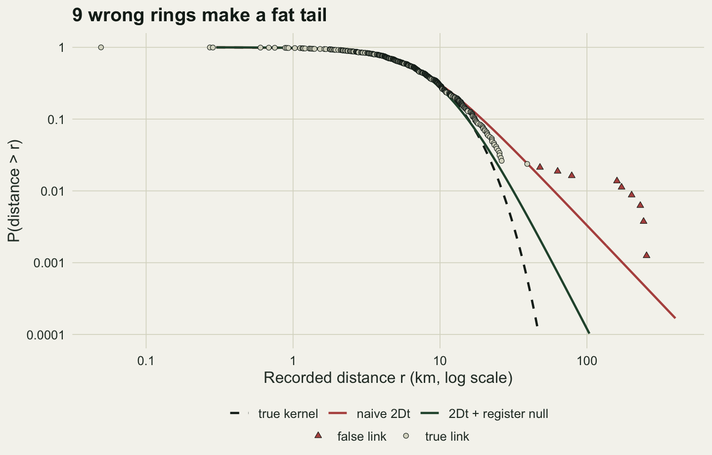
The tail exponent follows the join
Seven cells, 200 data sets each: the thin truth at the five harmful shares, and the fat truth at none and at 1 per cent. Every data set gets both naive fits, the 2Dt refitted with its farthest 5 per cent dropped, and both mixtures.
one_ds <- function(harm, truth) {
  ds <- make_ds(harm, truth)
  r_obs <- ds$r_obs
  fe <- fit_exp(r_obs)
  ft <- fit_2dt(r_obs)
  ftrim <- fit_2dt(r_obs[r_obs <= quantile(r_obs, 0.95)])
  me <- fit_mix_exp(r_obs, ds$dist_all)
  mt <- fit_mix_2dt(r_obs, ds$dist_all)
  far <- r_obs > far_km
  mid <- r_obs > mid_km & !far
  g_own <- exp(-r_obs / me$a)
  f_null <- rowMeans(exp(-ds$dist_all / me$a))
  me_post <- me$lam * f_null / ((1 - me$lam) * g_own + me$lam * f_null)
  c(harm = mean(ds$harmful), relinked = mean(ds$relinked),
    n_far = sum(far), n_far_false = sum(far & ds$harmful),
    t_wins = as.numeric(-2 * ft$ll + 4 < -2 * fe$ll + 2),
    true_mean = mean(ds$moved), naive_mean = mean(r_obs),
    naive_p = ft$p, trim_p = ftrim$p,
    me_lam = me$lam, me_mean = me$mean, me_post_far = sum(me_post[far]),
    me_post_mid = sum(me_post[mid]), me_post_all = sum(me_post),
    mt_lam = mt$lam, mt_p = mt$p, mt_mean = mt$mean)
}
cells <- data.frame(truth = c(rep("thin", 5), "fat", "fat"),
                    harm = c(0, 0.0025, 0.005, 0.01, 0.02, 0, 0.01))
per_ds <- vector("list", nrow(cells))
for (i in seq_len(nrow(cells))) {
  set.seed(32710 + i)
  m <- t(replicate(n_ds, one_ds(cells$harm[i], cells$truth[i])))
  per_ds[[i]] <- data.frame(truth = cells$truth[i], harm_set = cells$harm[i], m)
}
summ <- do.call(rbind, lapply(per_ds, function(d) data.frame(
  truth = d$truth[1], harm_set = d$harm_set[1],
  relinked = mean(d$relinked), harm = mean(d$harm),
  naive_p = median(d$naive_p), naive_p_lo = quantile(d$naive_p, 0.1),
  naive_p_hi = quantile(d$naive_p, 0.9),
  mt_p = median(d$mt_p), mt_p_lo = quantile(d$mt_p, 0.1), mt_p_hi = quantile(d$mt_p, 0.9),
  trim_p = median(d$trim_p), trim_ratio = median(d$trim_p / d$naive_p),
  trim_ratio_min = min(d$trim_p / d$naive_p),
  naive_mean = mean(d$naive_mean), true_mean = mean(d$true_mean),
  me_lam = mean(d$me_lam), me_lam_se = sd(d$me_lam) / sqrt(nrow(d)),
  mt_lam = mean(d$mt_lam), mt_lam_se = sd(d$mt_lam) / sqrt(nrow(d)),
  me_mean = mean(d$me_mean), mt_mean = median(d$mt_mean),
  far_false = sum(d$n_far_false) / sum(d$n_far), n_far = mean(d$n_far),
  t_wins = mean(d$t_wins))))
rownames(summ) <- NULL
th <- summ[summ$truth == "thin", ]
ft0 <- summ[summ$truth == "fat" & summ$harm_set == 0, ]
ft1 <- summ[summ$truth == "fat" & summ$harm_set == 0.01, ]
print(summ[, c("truth", "harm_set", "relinked", "harm", "naive_p", "mt_p",
               "naive_mean", "me_lam", "mt_lam")], digits = 3)
truth harm_set relinked harm naive_p mt_p naive_mean me_lam mt_lam
1 thin 0.0000 0.00000 0.00000 2.201 2.20 8.02 2.71e-05 4.78e-05
2 thin 0.0025 0.00264 0.00263 1.783 2.15 8.40 2.68e-03 2.34e-03
3 thin 0.0050 0.00539 0.00530 1.601 2.16 8.73 5.46e-03 5.08e-03
4 thin 0.0100 0.00996 0.00978 1.404 2.10 9.40 9.97e-03 9.41e-03
5 thin 0.0200 0.02031 0.02007 1.132 2.10 10.93 2.02e-02 1.94e-02
6 fat 0.0000 0.00000 0.00000 1.197 1.20 5.01 4.03e-03 1.27e-04
7 fat 0.0100 0.00983 0.00971 0.981 1.23 6.53 1.49e-02 1.00e-02The realised shares match the design: 0.00, 0.26, 0.53, 0.98, 2.01 per cent harmful across the thin cells, from re-link rates of 0.00, 0.26, 0.54, 1.00, 2.03 per cent.
With no false links, the naive 2Dt fitted to the thin truth reads a median tail exponent of 2.20: a 2Dt has no exponential tail, so this is simply what a clean thin sample of 400 looks like through that family. It is the reference value for the thin truth. Add harmful false links and the median falls to 1.78 at 0.25 per cent, 1.60 at 0.5, 1.40 at 1 and 1.13 at 2 per cent. The genuinely fat truth, fitted clean, gives 1.20 against its true 1.2. So at 2 per cent a thin kernel reads as fat-tailed as the fat one, and one false record in fifty is enough to do it. The spread across data sets does not rescue the naive reading: at 2 per cent the central 80 per cent of data sets run from 0.94 to 1.38, well below the clean thin interval of 1.81 to 2.74.
A fat truth is not protected either. With 1 per cent false links its naive exponent falls from 1.20 to 0.98, below 1, the value under which a 2Dt no longer has a finite variance of distance, and so into a tail heavier than anything the true kernel produces.
The 2Dt plus register null reads 2.20, 2.15, 2.16, 2.10, 2.10 across the five thin cells, and 1.20 and 1.23 for the fat truth at 0 and 1 per cent. Against the naive drop from 2.20 to 1.13, the mixture’s exponent barely moves, and its movement is small beside its own spread across data sets.
drift <- rbind(
  data.frame(harm = th$harm, p = th$naive_p, lo = th$naive_p_lo, hi = th$naive_p_hi,
             fit = "naive 2Dt"),
  data.frame(harm = th$harm, p = th$mt_p, lo = th$mt_p_lo, hi = th$mt_p_hi,
             fit = "2Dt + register null"))
drift$fit <- factor(drift$fit, levels = c("naive 2Dt", "2Dt + register null"))
drift$x <- 100 * drift$harm + ifelse(drift$fit == "naive 2Dt", -0.03, 0.03)
ref_lines <- data.frame(y = c(th$naive_p[1], fat_p),
                        lab = c("clean thin sample, naive reading", "fat truth, p = 1.2"))
ggplot(drift, aes(x, p, colour = fit)) +
  geom_hline(data = ref_lines, aes(yintercept = y), linetype = 2,
             colour = c(te_body, te_gold), linewidth = 0.5) +
  annotate("text", x = c(1.5, 0.6), y = ref_lines$y + c(0.07, -0.07), label = ref_lines$lab,
           hjust = 0.5, size = 3.3, colour = te_body) +
  geom_errorbar(aes(ymin = lo, ymax = hi), width = 0.05, linewidth = 0.5) +
  geom_line(linewidth = 0.6) +
  geom_point(size = 2.4) +
  scale_colour_manual(values = c("naive 2Dt" = te_rust, "2Dt + register null" = te_forest),
                      name = NULL) +
  labs(x = "Harmful false links (per cent of recoveries)", y = "Fitted tail exponent p",
       title = "The join picks the tail") +
  theme_datasheet() + theme(legend.position = "bottom")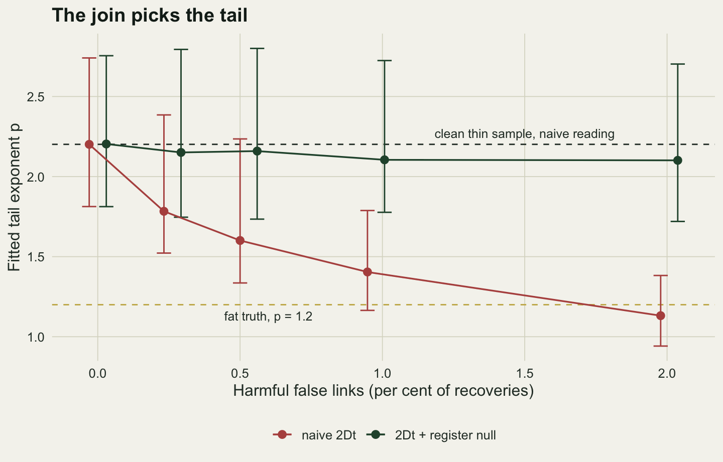
Two other numbers that a first look at such data would produce are pure arithmetic, and they are printed here as checks rather than findings.
set.seed(32720)
n_pair <- 1e6
pair_d <- sqrt((runif(n_pair, 0, side_km) - runif(n_pair, 0, side_km))^2 +
               (runif(n_pair, 0, side_km) - runif(n_pair, 0, side_km))^2)
p_far_pair <- mean(pair_d > far_km)
mean_pair <- mean(pair_d)
p_far_thin <- surv_exp2(far_km, thin_scale)
e_far <- n_rec * (th$harm * p_far_pair + p_far_thin)
aic_pred <- 1 - exp(-e_far)
aic_se <- sqrt(th$t_wins * (1 - th$t_wins) / n_ds)
mean_pred <- (1 - th$harm) * 8 + th$harm * mean_pair
far_pred <- th$harm * p_far_pair / (th$harm * p_far_pair + (1 - th$harm) * p_far_thin)
thin_false_ds <- do.call(rbind, per_ds[2:5])
thin_false_ds <- thin_false_ds[thin_false_ds$n_far_false > 0, ]
flip_false <- mean(thin_false_ds$t_wins)
clean_wins <- sum(per_ds[[1]]$t_wins)
clean_wins_nofar <- sum(per_ds[[1]]$t_wins == 1 & per_ds[[1]]$n_far == 0)
print(round(c(flip_given_false_far = flip_false, clean_wins = clean_wins,
              clean_wins_no_far = clean_wins_nofar), 3))
flip_given_false_far clean_wins clean_wins_no_far
0.987 10.000 10.000 print(round(rbind(far_false = th$far_false, far_closed = far_pred, aic_share = th$t_wins, aic_poisson = aic_pred,
naive_mean = th$naive_mean, mean_closed = mean_pred), 3)) [,1] [,2] [,3] [,4] [,5]
far_false 0.000 0.985 0.990 0.992 0.998
far_closed 0.000 0.980 0.990 0.995 0.997
aic_share 0.050 0.660 0.860 0.965 0.995
aic_poisson 0.020 0.629 0.862 0.974 0.999
naive_mean 8.017 8.403 8.735 9.402 10.927
mean_closed 8.000 8.390 8.787 9.452 10.982The share of recorded distances beyond 50 km that are false is 0.985, 0.990, 0.992, 0.998 at the four nonzero rates. That is set by the thin true tail, which puts a genuine record past 50 km with probability \(5.03 \times 10^{-5}\), against 0.93 for a random pair of points in the square; the closed form, the harmful share times 0.93 over itself plus the rest times \(5.03 \times 10^{-5}\), gives 0.980, 0.990, 0.995, 0.997. The share of data sets in which the 2Dt beats the exponential on AIC is 0.050, 0.660, 0.860, 0.965, 0.995 across the five cells (Monte Carlo standard errors up to 0.033), beside the Poisson chance of at least one record past 50 km, 0.020, 0.629, 0.862, 0.974, 0.999. One false far record is enough to flip the family: in the data sets holding at least one, the 2Dt wins in 98.7 per cent. The clean cell runs above its Poisson figure for another reason: the 2Dt wins there in 10 data sets, and 10 of them hold no record past 50 km at all, so the shape of the bulk decides those and the Poisson figure does not count them. The naive mean distance is also closed form: a false record carries the mean distance between two random points in the square, 156.6 km, so the expected mean is (1 - lambda) times 8 plus lambda times 156.6, which gives 10.98 km at the realised 2 per cent against a measured 10.93 km, a rise of 37 per cent over the true mean of 7.97 km. None of these needs a simulation. The exponent drift above does, because a likelihood fit spreads a few far records over the shape of the whole curve.
Dropping the farthest records
The obvious defence is the one the kernel-checking post offers: drop the farthest 5 per cent and refit, and if the exponent jumps, the tail was resting on a handful of points. It was run on every data set above.
trim_ratio <- function(d) d$trim_p / d$naive_p
tr_thin2 <- trim_ratio(per_ds[[5]])
tr_fat0 <- trim_ratio(per_ds[[6]])
tr_thin0 <- trim_ratio(per_ds[[1]])
jump_rule <- 1.5
share_jump <- c(thin2 = mean(tr_thin2 > jump_rule), fat0 = mean(tr_fat0 > jump_rule),
                thin0 = mean(tr_thin0 > jump_rule))
p_order <- mean(outer(tr_thin2, tr_fat0, ">"))
p_order0 <- mean(outer(tr_thin2, tr_thin0, ">"))
print(round(rbind(median = c(median(tr_thin2), median(tr_fat0), median(tr_thin0)),
                  minimum = c(min(tr_thin2), min(tr_fat0), min(tr_thin0)),
                  share_over_rule = share_jump), 3))
thin2 fat0 thin0
median 3.334 1.968 2.558
minimum 1.880 1.489 1.655
share_over_rule 1.000 0.995 1.000The check fires on nearly every data set. Taking a rise of more than half in the exponent as a jump, it flags 100.0 per cent of the thin data sets with 2 per cent false links, 99.5 per cent of the clean fat data sets, and 100.0 per cent of the clean thin ones. The smallest ratio of trimmed to full exponent in any of the three cells is 1.49. Dropping the farthest 5 per cent and refitting without a truncation term steepened the tail in every one of these data sets, because the refit treats a sample cut at its 95th percentile as if it were complete. As written, the check cannot come out “barely moves” on these data: the jump is the bias of fitting a truncated sample as if it were whole, the bias that Check 2 of the kernel-checking post warns about for trap windows.
The size of the jump does differ. The median ratio is 3.33 with false links on the thin truth against 1.97 on the clean fat truth, and a data set from the first cell jumps further than one from the second in 98 per cent of pairs. But a clean thin sample jumps by a median 2.56, and the false-link cell beats it in only 70 per cent of pairs. The size of the jump grows both with how thin the bulk of the kernel is and with the false far records: the clean fat truth jumps least, the clean thin truth more, and the same thin truth with false links more again. With one data set in hand and no reference cell to compare against, the analyst cannot tell which of the two made a given jump, and so the check cannot say which far points the join put there.
A null built from the register
The mixture needs no threshold. It asks of each record how likely its recovery location is under its own ringing site and how likely it is under a random site from the register, and it lets the data set the weight between the two.
lam_ratio_thin <- th$mt_lam[-1] / th$relinked[-1]
lam_ratio_fat <- ft1$mt_lam / ft1$relinked
print(round(rbind(harm = summ$harm, relinked = summ$relinked, lam_exp_null = summ$me_lam, se_exp = summ$me_lam_se,
                  lam_2dt_null = summ$mt_lam, se_2dt = summ$mt_lam_se,
                  mean_exp_null = summ$me_mean, mean_2dt_null = summ$mt_mean), 4))
[,1] [,2] [,3] [,4] [,5] [,6] [,7]
harm 0.0000 0.0026 0.0053 0.0098 0.0201 0.0000 0.0097
relinked 0.0000 0.0026 0.0054 0.0100 0.0203 0.0000 0.0098
lam_exp_null 0.0000 0.0027 0.0055 0.0100 0.0202 0.0040 0.0149
se_exp 0.0000 0.0002 0.0003 0.0004 0.0005 0.0003 0.0004
lam_2dt_null 0.0000 0.0023 0.0051 0.0094 0.0194 0.0001 0.0100
se_2dt 0.0000 0.0002 0.0003 0.0004 0.0005 0.0000 0.0003
mean_exp_null 8.0151 8.0101 7.9478 7.9695 7.9772 4.8457 4.8236
mean_2dt_null 8.1190 8.1080 8.0691 8.1123 8.0861 5.0148 4.9838On the thin truth, the exponential plus register null returns a mean false share of 0.0000, 0.0027, 0.0055, 0.0100, 0.0202 against its target, the realised re-link rate, of 0.0000, 0.0026, 0.0054, 0.0100, 0.0203 (Monte Carlo standard errors up to 0.0005), and a mean distance of 7.95 to 8.02 km against the true 8. The 2Dt plus register null returns 0.0000, 0.0023, 0.0051, 0.0094, 0.0194, that is 0.89 to 0.95 of the realised re-link rate at the nonzero rates, and a median mean distance of 8.07 to 8.12 km. The small shortfall fits the fat family giving the kernel a heavier tail than an exponential has, so that the nearest false records are partly credited to movement.
The case that matters is the fat truth, where real long moves and false links both produce far records. With 1 per cent harmful false links (realised 0.0097), the 2Dt plus register null returns a mean false share of 0.0100 (Monte Carlo standard error 0.0003), a ratio of 1.02 to the realised re-link rate of 0.0098, with a median exponent of 1.23 (central 80 per cent 1.06 to 1.37) and a median mean distance of 4.98 km against 5.01. The naive mean distance in that cell is 6.53 km. With no false links the same mixture returns a false share of 0.00013 and an exponent of 1.20.
The price: a thin family inside the mixture
The register null can tell a false link from a real long move only through the kernel. A far record is judged false if the kernel makes it less likely than a random site would, so a kernel with too thin a tail judges many real long movers false.
fat0_ds <- per_ds[[6]]
fat1_ds <- per_ds[[7]]
fail_lam0 <- mean(fat0_ds$me_lam)
fail_lam0_q <- quantile(fat0_ds$me_lam, c(0.1, 0.9))
fail_lam1 <- mean(fat1_ds$me_lam)
fail_excess <- fail_lam1 - ft1$relinked
fail_mean0 <- ft0$me_mean
real_far0 <- ft0$n_far
post_far <- mean(fat0_ds$me_post_far)
post_far_share <- sum(fat0_ds$me_post_far) / sum(fat0_ds$n_far)
post_mid <- mean(fat0_ds$me_post_mid)
post_all <- mean(fat0_ds$me_post_all)
print(round(c(post_far = post_far, post_far_share = post_far_share, post_mid = post_mid,
              post_all = post_all, n_times_lam = n_rec * fail_lam0), 3))
post_far post_far_share post_mid post_all n_times_lam
0.776 0.760 0.782 1.614 1.611 print(round(c(exp_null_lam_0 = fail_lam0, q10 = fail_lam0_q[[1]], q90 = fail_lam0_q[[2]],
twodt_null_lam_0 = ft0$mt_lam, exp_null_lam_1 = fail_lam1,
harm_1 = ft1$harm, exp_null_mean_0 = fail_mean0,
real_far_records = real_far0), 4)) exp_null_lam_0 q10 q90 twodt_null_lam_0
0.0040 0.0000 0.0081 0.0001
exp_null_lam_1 harm_1 exp_null_mean_0 real_far_records
0.0149 0.0097 4.8457 1.0200 Fitted to the fat truth with no false links at all, the exponential plus register null returns a mean false share of 0.0040 (central 80 per cent of data sets 0.0000 to 0.0081), where the 2Dt version on the same data returns 0.00013. That is 1.6 records per data set declared false where none are; the clean fat data sets hold on average 1.02 genuine records beyond 50 km. Record by record, the fitted probability that a link is false puts 0.78 records per data set beyond 50 km down as false, 76 per cent of the genuine long movers, and another 0.78 among the moves of 20 to 50 km; the moderately long moves carry about as much of the written-off dispersal as the long ones. Its mean distance is 4.85 km against 5.01. With 1 per cent false links it returns 0.0149, overshooting the realised re-link rate by 0.0051, the same order as the 0.0040 it finds with no false links: absorbed real dispersal on top of the false links.
That is the honest price of the repair. The mixture removes whatever the kernel inside it cannot explain, so it can only be trusted to remove the join’s records if the kernel is allowed a tail at least as fat as the birds’. The fat family costs little when the truth is thin, as the section above shows; the thin family costs real dispersal when the truth is fat.
lam_long <- do.call(rbind, lapply(per_ds, function(d) rbind(
  data.frame(truth = d$truth, harm_set = d$harm_set, lam = d$me_lam, fit = "exponential + null"),
  data.frame(truth = d$truth, harm_set = d$harm_set, lam = d$mt_lam, fit = "2Dt + null"))))
lam_long$cell <- factor(sprintf("%s kernel, %.2f%%", lam_long$truth, 100 * lam_long$harm_set),
                        levels = unique(sprintf("%s kernel, %.2f%%", cells$truth, 100 * cells$harm)))
lam_long$fit <- factor(lam_long$fit, levels = c("exponential + null", "2Dt + null"))
harm_ref <- data.frame(cell = levels(lam_long$cell), harm = summ$harm)
harm_ref$cell <- factor(harm_ref$cell, levels = levels(lam_long$cell))
ggplot(lam_long, aes(cell, 100 * lam, fill = fit)) +
  geom_boxplot(outlier.size = 0.5, linewidth = 0.3, colour = te_ink,
               position = position_dodge(width = 0.8), width = 0.7) +
  geom_errorbar(data = harm_ref, aes(x = cell, ymin = 100 * harm, ymax = 100 * harm),
                inherit.aes = FALSE, width = 0.85, linewidth = 1, colour = te_rust) +
  scale_fill_manual(values = c("exponential + null" = te_gold, "2Dt + null" = te_forest),
                    name = NULL) +
  labs(x = NULL, y = "Estimated false links (per cent)",
       title = "A thin family eats real dispersal") +
  theme_datasheet() +
  theme(legend.position = "bottom", axis.text.x = element_text(angle = 30, hjust = 1))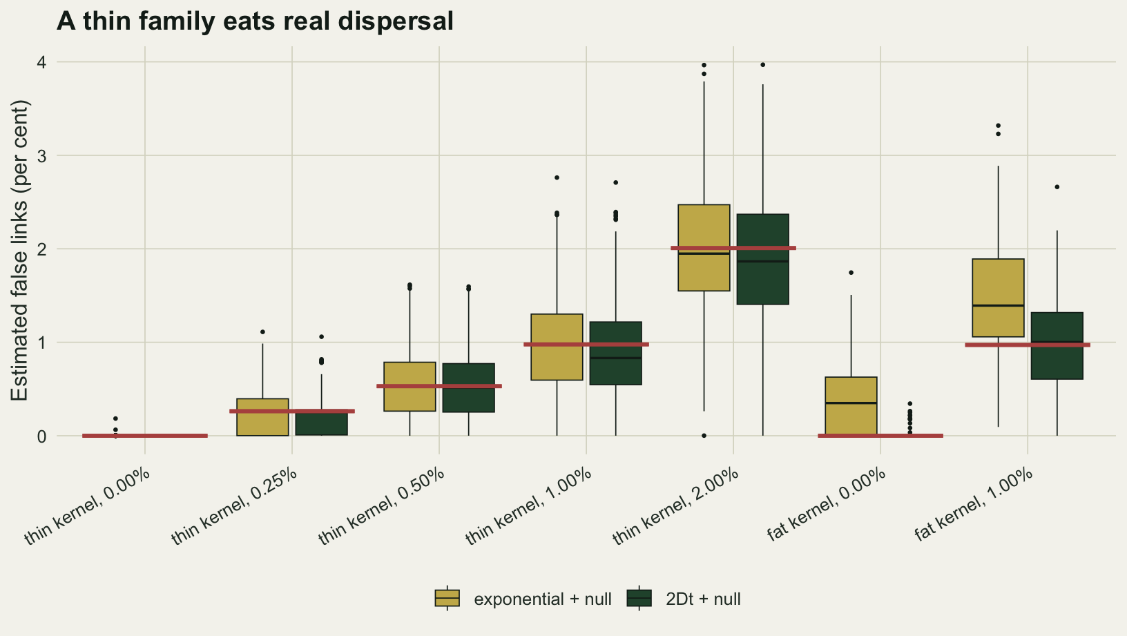
Colonial species
Seabirds and colonial waders are ringed at colonies and recovered, very often, at colonies. A bird that stays is recovered at distance zero, and a bird that moves is recovered at another colony, so the recorded distances take only the values of the colony-to-colony distances. Here the ringing sites are the colonies: a bird stays with probability 0.6 and otherwise moves to another colony with probability proportional to the 2Dt kernel at that distance, with the same a and p as the fat truth. The fitted model is the same discrete kernel plus a register null, in which a false link makes the recorded colony independent of the ringing colony and the recovery colony has its marginal probability under a random ringing site.
move_mat <- function(d2_col, stay, a, p) {
  wt <- exp(-(p + 1) * log1p(d2_col / a^2))
  diag(wt) <- 0
  pm <- (1 - stay) * wt / rowSums(wt)
  diag(pm) <- stay
  pm
}
one_col <- function(harm, continuous = FALSE) {
  link_rate <- harm * n_site / (n_site - 1)
  sx <- runif(n_site, 0, side_km)
  sy <- runif(n_site, 0, side_km)
  d2_col <- outer(sx, sx, "-")^2 + outer(sy, sy, "-")^2
  pm <- move_mat(d2_col, 0.6, fat_a, fat_p)
  origin <- sample.int(n_site, n_rec, replace = TRUE)
  cum_p <- t(apply(pm, 1, cumsum))
  found <- 1L + rowSums(runif(n_rec) > cum_p[origin, , drop = FALSE])
  relinked <- runif(n_rec) < link_rate
  link <- origin
  link[relinked] <- sample.int(n_site, sum(relinked), replace = TRUE)
  nll <- function(th, mix) {
    pm_h <- move_mat(d2_col, plogis(th[1]), exp(th[2]), exp(th[3]))
    lam_h <- if (mix) plogis(th[4]) else 0
    -sum(log((1 - lam_h) * pm_h[cbind(link, found)] + lam_h * colMeans(pm_h)[found]))
  }
  o_naive <- optim(c(0, log(fat_a), log(fat_p)), nll, mix = FALSE,
                   method = "Nelder-Mead", control = list(maxit = 2000))
  o_mix <- optim(c(o_naive$par, qlogis(0.01)), nll, mix = TRUE,
                 method = "Nelder-Mead", control = list(maxit = 3000))
  r_own <- pmax(sqrt(d2_col[cbind(link, found)]), 1e-3)
  out <- c(harm = mean(relinked & link != origin), naive_p = exp(o_naive$par[3]),
           mix_p = exp(o_mix$par[3]), mix_lam = plogis(o_mix$par[4]),
           stay_hat = plogis(o_mix$par[1]), stayed = mean(r_own < 1))
  if (continuous) {
    cont <- fit_mix_2dt(r_own, sqrt(d2_col[found, , drop = FALSE]))
    out <- c(out, cont_lam = cont$lam, cont_p = cont$p)
  }
  out
}
col_ds <- lapply(c(0, 0.01), function(h) {
  set.seed(32790 + round(1e4 * h))
  data.frame(harm_set = h, t(replicate(n_ds, one_col(h))))
})
col_sum <- do.call(rbind, lapply(col_ds, function(d) data.frame(
  harm_set = d$harm_set[1], harm = mean(d$harm), naive_p = median(d$naive_p),
  mix_p = median(d$mix_p), mix_p_lo = quantile(d$mix_p, 0.1),
  mix_p_hi = quantile(d$mix_p, 0.9), mix_lam = mean(d$mix_lam),
  mix_lam_se = sd(d$mix_lam) / sqrt(nrow(d)), stay_hat = median(d$stay_hat),
  stayed = mean(d$stayed))))
rownames(col_sum) <- NULL
col0 <- col_sum[1, ]
col1 <- col_sum[2, ]
n_cont <- 25L
set.seed(32799)
cont_ds <- data.frame(t(replicate(n_cont, one_col(0, continuous = TRUE))))
cont_lam_q <- quantile(cont_ds$cont_lam, c(0, 0.5))
cont_p_min <- min(cont_ds$cont_p)
cont_n_one <- sum(1 - cont_ds$cont_lam <= .Machine$double.eps)
print(col_sum, digits = 3)
harm_set harm naive_p mix_p mix_p_lo mix_p_hi mix_lam mix_lam_se stay_hat
1 0.00 0.0000 1.233 1.25 1.05 1.61 0.000522 0.000107 0.600
2 0.01 0.0107 0.961 1.22 1.01 1.54 0.010873 0.000477 0.599
stayed
1 0.600
2 0.592print(signif(c(cont_lam_min = cont_lam_q[[1]], cont_lam_median = cont_lam_q[[2]],
cont_p_min = cont_p_min, cont_n_one = cont_n_one), 3)) cont_lam_min cont_lam_median cont_p_min cont_n_one
1.00e+00 1.00e+00 4.01e+76 2.50e+01 The naive discrete fit reads a median exponent of 1.23 with no false links and 0.96 with 1 per cent (realised 0.0107). The discrete mixture reads 1.25 and 1.22 (central 80 per cent at 1 per cent: 1.01 to 1.54), against the true 1.2, and a mean false share of 0.0005 and 0.0109 (Monte Carlo standard error 0.0005). The repair carries over to colonies, provided it is written in the discrete form.
The continuous form does not carry over, and it is expensive to show, so it was run on 25 data sets with no false links. Fed the colony-to-colony distances, the 2Dt plus register null from the sections above returns a false share of 1 to machine precision in 25 of the 25 data sets, with a fitted exponent of at least \(4.0 \times 10^{76}\): the fit has run off the edge of the parameter space (the exact runaway depends on how zero distances are floored; the likelihood has no maximum either way). About 60 per cent of the records sit at distance zero, a point mass that no density over the plane can carry, and the register null, which has a site at every colony where a bird is found, absorbs everything. A colonial analysis needs the kernel over colonies, not a density over the plane.
col_long <- do.call(rbind, lapply(col_ds, function(d) rbind(
  data.frame(harm_set = d$harm_set, p = d$naive_p, fit = "naive discrete kernel"),
  data.frame(harm_set = d$harm_set, p = d$mix_p, fit = "discrete kernel + register null"))))
col_long$fit <- factor(col_long$fit, levels = c("naive discrete kernel",
                                                "discrete kernel + register null"))
col_long$cell <- factor(ifelse(col_long$harm_set == 0, "no false links", "1% false links"),
                        levels = c("no false links", "1% false links"))
ggplot(col_long, aes(cell, p, fill = fit)) +
  geom_hline(yintercept = fat_p, linetype = 2, colour = te_body, linewidth = 0.5) +
  geom_boxplot(outlier.size = 0.5, linewidth = 0.3, colour = te_ink, width = 0.6,
               position = position_dodge(width = 0.75)) +
  scale_fill_manual(values = c("naive discrete kernel" = te_rust,
                               "discrete kernel + register null" = te_forest), name = NULL) +
  labs(x = NULL, y = "Fitted tail exponent p", title = "Colonies need the discrete form") +
  theme_datasheet() + theme(legend.position = "bottom")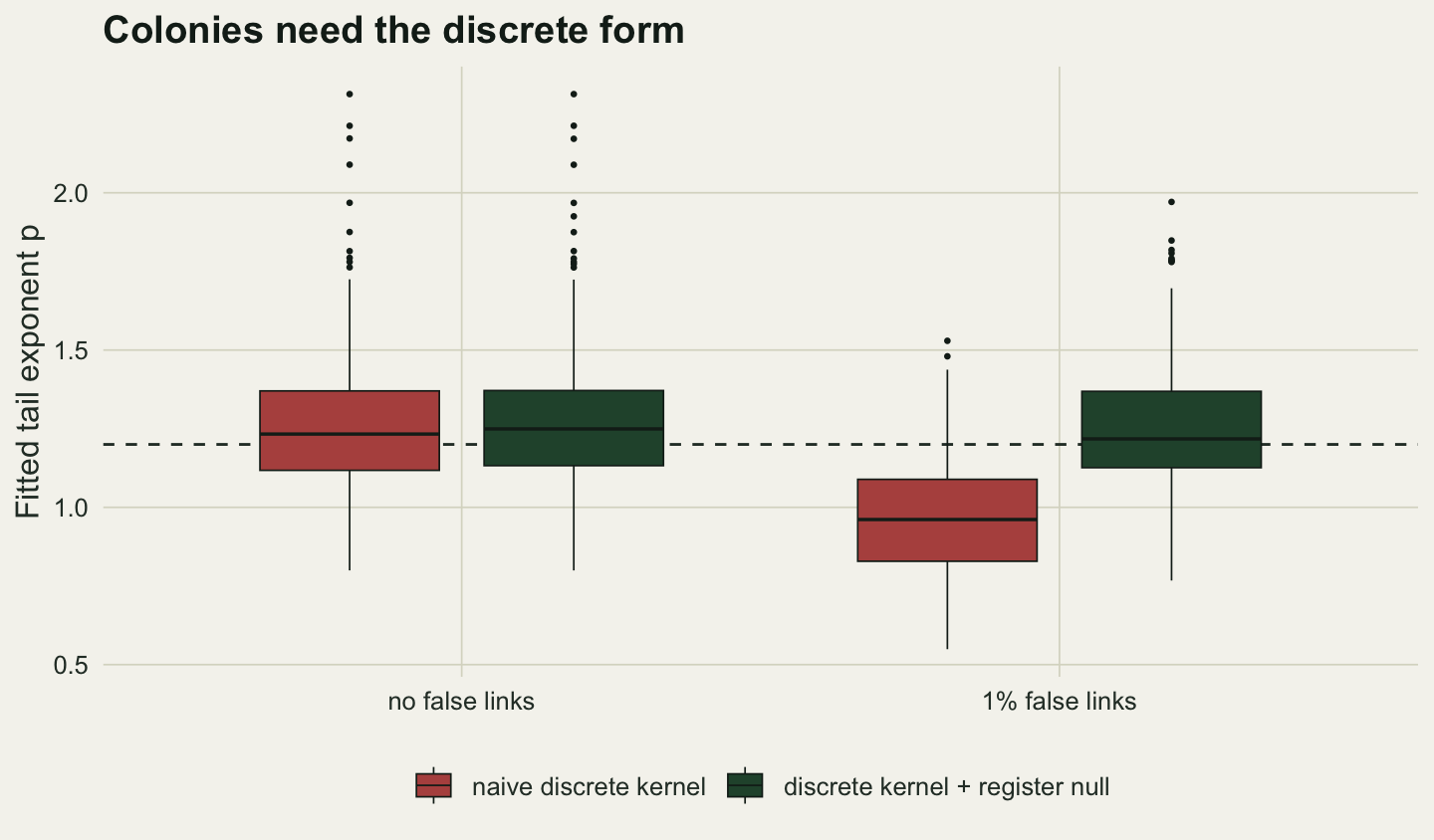
What to report
A dispersal analysis built on ring recoveries joined to a register should say how the ring number was checked and what happened to numbers that did not match. The count of numbers rejected because they were never issued is the one direct measure of misreading that every scheme already holds. The harmful share is smaller than the misread rate: only misreads that form another issued number pass the register, and only those that land on another site’s ring move the distance. How much smaller depends on how a scheme issues its rings, in series of consecutive numbers to ringers who work in one place, and on species and date checks at the time of acceptance; the simulation here set the harmful share directly because that conversion needs a scheme’s own numbers.
Then fit the register mixture beside the naive fit, and report the false share it estimates, the exponent under both fits, and the mean distance under both. The null needs the register’s weights by site and the share of recoveries by site, not just the list of sites: here every site issued the same number of rings and every ringed bird had the same chance of recovery, and a register with a few large sites puts most of the null’s mass near them. Put a fat-tailed family inside the mixture, because a false share estimated with a thin family runs high by the real long movers it absorbs. If the species is colonial, write the kernel over the colonies.
A tail that turns fat only through a handful of the farthest records is a reason to look those records up in the register before it is a reason to write about long-distance dispersal.
Honest limits
False links here land uniformly on the register. Real misreads cluster: a misread last digit keeps the number within its own series, and where a series goes to one ringer at one site, such a misread links to the same or a nearby site and does little harm, while a misread early digit can jump to a distant ringer. The register null as written assumes the uniform case; a scheme that knows its confusion structure would weight the null by it.
The null as written weights sites by rings issued, which is right only when every ringed bird has the same chance of being recovered. If recovery effort is concentrated where ringing is (ringers find their own birds), that fails. The recovery location of a falsely linked bird then follows the sites that recovered birds come from, which can be estimated from the linked records themselves, while the wrong site still follows the register. With pi_s the share of recoveries from site s, the likelihood of a record linked to site L becomes
[(1 - lambda) pi_L k(x_i - s_L) + lambda w_L sum_s pi_s k(x_i - s)] / [(1 - lambda) pi_L + lambda w_L]
so the two weights enter separately and the mixing weight differs by site; with pi_s = w_s it reduces to the formula above. The same effort surface also bends the kernel that the true links show, in the naive and the mixture fits alike, and that is not corrected here.
The kernel families inside the mixture are the two that also generated the data. A real kernel is neither, and a 2Dt fitted to a kernel with a different tail shape will again give the null whatever it cannot fit. The fat family is the safer of the two here, not a guarantee.
The geometry is one square with 60 sites and 400 recoveries. The drift depends on the ratio of region size to kernel scale: in a smaller region, false records land less far out and change the exponent less.
The same wrong-partner error arises in seed parentage, when a seedling is assigned to the wrong mother; when the mother is taken to be the nearest adult, the wrong partner is the closest one available and the distances shrink rather than fatten, which Seed dispersal: the nearest adult is not the parent derives; a wrong mother picked at random among the candidates, as weak genetic exclusion can do, was not simulated for either post.
References
Paradis E, Baillie SR, Sutherland WJ, Gregory RD 1998 Journal of Animal Ecology 67(4):518-536 (10.1046/j.1365-2656.1998.00215.x)
Neter J, Maynes ES, Ramanathan R 1965 Journal of the American Statistical Association 60(312):1005-1027 (10.1080/01621459.1965.10480846)
Lahiri P, Larsen MD 2005 Journal of the American Statistical Association 100(469):222-230 (10.1198/016214504000001277)