library(ggplot2)
library(patchwork)

te_paper  <- "#f5f4ee"
te_ink    <- "#16241d"
te_body   <- "#2c3a31"
te_forest <- "#275139"
te_rust   <- "#b5534e"
te_gold   <- "#c9b458"
te_line   <- "#dad9ca"

theme_datasheet <- function() {
  theme_minimal(base_size = 12) +
    theme(plot.background  = element_rect(fill = te_paper, colour = NA),
          panel.background = element_rect(fill = te_paper, colour = NA),
          panel.grid.major = element_line(colour = te_line, linewidth = 0.3),
          panel.grid.minor = element_blank(),
          text             = element_text(colour = te_body),
          plot.title       = element_text(colour = te_ink, face = "bold"),
          plot.subtitle    = element_text(colour = te_body),
          axis.text        = element_text(colour = te_body))
}Misread colour rings and apparent survival
R
capture-recapture
survival
colour ringing
simulation
ecology tutorial
Misread colour rings revive dead birds as resightings: in R, CJS survival bias grows with study length and a two-sighting filter fails when sightability varies.
A shorebird team has been colour-ringing godwits on the same meadows for ten years. Every bird carries a unique combination of coloured rings, and every spring volunteers with telescopes read those combinations off birds feeding on the mudflats, a few hundred metres away, often in wind and low light. Each reading is typed in and looked up in the ring register. If the combination is in the register, the sighting joins that bird’s capture history; if it is not, the record is thrown out as an obvious error. The survival analysis then runs a Cormack-Jolly-Seber (CJS) model on the joined histories.
The weak point is the join. A misread combination that happens to form another code the scheme has issued passes the register check, and it becomes a sighting of a bird that was not there. The register holds every bird ever ringed, including the ones that died years ago, so some of these sightings bring dead birds back to life for a season. This is known. Tucker and colleagues measured misread rates in a ten-year Red Knot flag dataset and showed by simulation that misreads produce spurious negative trends in survival over time, worst in long studies, and that dropping every flag reported only once in a sampling occasion reduced the bias and removed the spurious trend, at a cost in precision. Rakhimberdiev and colleagues report systematic positive biases in CJS survival from misread resightings and fix them with a model that splits each season into secondary resighting sessions and uses the repeated sightings within it. This post is a demonstration of their result in a constant-parameter CJS model, not a claim to it. What is measured here is narrower: how the bias grows with the number of seasons, what happens to the filter they evaluated when birds differ in how often they are seen, and whether a detection probability for the dead state, added to a two-class detection mixture in an ordinary CJS model, can do the filter’s job without secondary sessions.
Cormack-Jolly-Seber survival models in R builds the m-array likelihood reused below, and it says that apparent survival “is a lower bound on true survival”, because a dead bird and an emigrant look the same. That is right as long as every sighting is real. Once the resightings are joined to the ring register by a code that can be misread, some sightings belong to birds that are already dead, the bound fails, and the failure grows with every season the study runs. Joint live-dead models proves the downward version exactly: apparent survival is survival times fidelity. Misreads push the other way.
The same error appears on the site in a closed population. Identification errors in capture-recapture measures missed and false photo matches under model M0 and leaves out the case of a photograph filed under a different catalogued animal, because M0 uses only the number of entries and captures and that error barely moves it. In an open model it is the whole problem. The nearest method post is Transients and the single-capture rule in CJS, where a deletion rule biases survival and a model does better; the filter here looks like the opposite case, a rule that fixes survival, and the question is when it stops doing so. The repair used at the end is the event layer of Multi-event models for uncertain states applied to the dead state, combined with the two-class detection mixture that Capture heterogeneity: Mt, Mb and Mh in R fits in a closed population.
A ring register that keeps the dead
Each simulated study rings 80 birds a season for the first K - 1 seasons and resights in seasons 2 to K. A bird survives each interval with probability 0.85, the same for every bird and every year. While it is alive it is read a Poisson number of times per season with mean 2. Each reading is misread with probability e, and half of all misreads (q = 0.5) form a combination that exists in the register; the other half are caught by the register check and discarded, so they do no harm. A misread that passes lands on a code drawn uniformly from every code issued so far, alive or dead. The season is scored as a detection when the joined readings for a code reach a threshold: one reading for the usual analysis, two for the filter. All of these constants are fixed before any run below.
phi_true <- 0.85
n_mark <- 80L
lam_mean <- 2
q_valid <- 0.5

sim_counts <- function(K, e, cv = 0, phi = phi_true, R = n_mark,
                       lam = lam_mean, q = q_valid) {
  N <- R * (K - 1)
  rel <- rep(seq_len(K - 1), each = R)
  last <- rel + rgeom(N, 1 - phi)
  lam_i <- if (cv > 0) rgamma(N, 1 / cv^2, scale = lam * cv^2) else rep(lam, N)
  cnt <- matrix(0L, N, K)
  cnt0 <- matrix(0L, N, K)
  fh <- data.frame(t = 2:K, n_false = 0, on_dead = 0, dead_codes = 0,
                   dead_seen = 0, n_alive = 0, issued = 0, live_seen1 = 0,
                   live_seen2 = 0, lam_alive = 0, n_reject = 0)
  for (tt in 2:K) {
    alive <- which(rel < tt & last >= tt)
    issued <- which(rel <= tt)
    n_read <- rpois(length(alive), lam_i[alive])
    n_mis <- rbinom(length(alive), n_read, e)
    cc <- integer(N)
    cc[alive] <- n_read - n_mis
    n_valid <- rbinom(1, sum(n_mis), q)
    hit <- integer(0)
    if (n_valid > 0) {
      hit <- issued[sample.int(length(issued), n_valid, replace = TRUE)]
      cc <- cc + tabulate(hit, nbins = N)
    }
    dead <- which(rel < tt & last < tt)
    fh[tt - 1, ] <- c(tt, n_valid, sum(last[hit] < tt), length(dead),
                      sum(cc[dead] >= 1), length(alive), length(issued),
                      sum(cc[alive] >= 1), sum(cc[alive] >= 2), sum(lam_i[alive]),
                      sum(n_mis) - n_valid)
    cnt[, tt] <- cc
    cnt0[alive, tt] <- n_read
  }
  cnt[cbind(seq_len(N), rel)] <- 99L
  cnt0[cbind(seq_len(N), rel)] <- 99L
  list(cnt = cnt, cnt0 = cnt0, fh = fh)
}

hist_of <- function(cnt, rule) (cnt >= rule) * 1L
The ringing occasion itself is coded as a certain detection, so a bird always enters its history at release. Every study is scored twice: cnt holds the readings as the register join delivers them, and cnt0 holds the same readings of the same birds as if every one had been read correctly. The no-misread controls below are therefore paired with the misread analyses bird for bird, and a difference between them is the effect of misreads alone. The fh table records, season by season, the truth that an analyst never sees: how many false hits there were, how many fell on dead codes, and how many dead codes were scored as seen.
The analysis side has two engines. The first is the constant survival, constant detection CJS model fitted by maximum likelihood to the m-array, with a Wald interval on the logit scale: the model of the CJS post, in the m-array form of Lebreton and colleagues. The second is a forward algorithm over individual histories, collapsed to unique histories with counts as weights, which allows two things the m-array cannot hold: a mixture of two detection classes, and a dead state that is itself “detected” with probability f.
marray_of <- function(H) {
  K <- ncol(H)
  pos <- which(H == 1L, arr.ind = TRUE)
  pos <- pos[order(pos[, 1], pos[, 2]), , drop = FALSE]
  same_bird <- c(pos[-1, 1] == pos[-nrow(pos), 1], FALSE)
  from <- pos[, 2]
  to <- c(pos[-1, 2], NA)
  to[!same_bird] <- K + 1L
  keep <- from < K
  m <- matrix(0, K - 1, K)
  m[] <- table(factor(from[keep], 1:(K - 1)), factor(to[keep] - 1L, 1:K))
  m
}

fit_marray <- function(m) {
  K1 <- nrow(m)
  ii <- row(matrix(0, K1, K1)); jj <- col(matrix(0, K1, K1))
  up <- jj >= ii
  gap <- (jj - ii + 1)[up]
  m_up <- m[, 1:K1][up]
  never <- m[, K1 + 1]
  nll <- function(th) {
    ph <- plogis(th[1]); pp <- plogis(th[2])
    pr <- matrix(0, K1, K1)
    pr[up] <- ph^gap * (1 - pp)^(gap - 1) * pp
    chi <- pmax(1 - rowSums(pr), 1e-300)
    -(sum(m_up * log(pr[up])) + sum(never * log(chi)))
  }
  o <- optim(c(1, 0), nll, method = "BFGS", hessian = TRUE)
  se <- sqrt(diag(solve(o$hessian)))
  c(phi = plogis(o$par[1]), p = plogis(o$par[2]),
    lo = plogis(o$par[1] - 1.96 * se[1]), hi = plogis(o$par[1] + 1.96 * se[1]))
}

collapse_hist <- function(H) {
  key <- apply(H, 1, paste, collapse = "")
  u <- !duplicated(key)
  list(H = H[u, , drop = FALSE], w = as.vector(table(key)[key[u]]))
}

lik_rows <- function(H, first, ph, pa, f) {
  a <- rep(1, nrow(H)); d <- rep(0, nrow(H))
  for (tt in 2:ncol(H)) {
    act <- first < tt
    y <- H[, tt]
    d <- ifelse(act, (d + a * (1 - ph)) * (y * f + (1 - y) * (1 - f)), d)
    a <- ifelse(act, a * ph * (y * pa + (1 - y) * (1 - pa)), a)
  }
  a + d
}

fit_hmm <- function(H, model, hess = FALSE) {
  cl <- collapse_hist(H)
  Hu <- cl$H; w <- cl$w
  first <- max.col(Hu, ties.method = "first")
  nll <- switch(model,
    one = function(th)
      -sum(w * log(lik_rows(Hu, first, plogis(th[1]), plogis(th[2]), 0) + 1e-300)),
    two = function(th) {
      ph <- plogis(th[1]); mw <- plogis(th[4])
      -sum(w * log(mw * lik_rows(Hu, first, ph, plogis(th[2]), 0) +
                   (1 - mw) * lik_rows(Hu, first, ph, plogis(th[3]), 0) + 1e-300))
    },
    twof = function(th) {
      ph <- plogis(th[1]); mw <- plogis(th[4]); f <- plogis(th[5])
      -sum(w * log(mw * lik_rows(Hu, first, ph, plogis(th[2]), f) +
                   (1 - mw) * lik_rows(Hu, first, ph, plogis(th[3]), f) + 1e-300))
    })
  init <- switch(model, one = c(1.5, 1.5), two = c(1.5, 1.5, -1, 0),
                  twof = c(1.5, 1.5, -1, 0, -4))
  o <- optim(init, nll, method = "BFGS", hessian = hess, control = list(maxit = 300))
  out <- c(phi = plogis(o$par[1]), conv = o$convergence)
  if (model == "twof") out <- c(out, f = plogis(o$par[5]))
  if (hess) {
    v <- tryCatch(diag(solve(o$hessian))[1], error = function(z) NA_real_)
    se <- if (is.finite(v) && v > 0) sqrt(v) else NA_real_
    out <- c(out, lo = plogis(o$par[1] - 1.96 * se), hi = plogis(o$par[1] + 1.96 * se))
  }
  out
}

set.seed(2909)
check_sim <- sim_counts(10, 0.03)
check_h <- hist_of(check_sim$cnt, 1)
check_marray <- fit_marray(marray_of(check_h))[["phi"]]
check_forward <- fit_hmm(check_h, "one")[["phi"]]
The two engines agree where they should. On one simulated ten-season study, the m-array fit gives an apparent survival of 0.85159 and the forward algorithm with one detection class and f fixed at zero gives 0.85158.
Apparent survival climbs with every season
The first block runs the constant CJS model on studies of 5, 10 and 15 seasons, with no misreads, with a misread rate of 3 per cent, and at 15 seasons also with 1 per cent. Every study is also scored under the two-sighting filter, so the next section compares the two analyses on the same simulated birds.
n_study_a <- 400L
cells_a <- data.frame(K = c(5, 10, 15, 15), e = c(0.03, 0.03, 0.03, 0.01))
set.seed(4417)
runs_a <- lapply(seq_len(nrow(cells_a)), function(g) {
  fits <- vector("list", n_study_a); truth <- vector("list", n_study_a)
  for (i in seq_len(n_study_a)) {
    s <- sim_counts(cells_a$K[g], cells_a$e[g])
    fits[[i]] <- c(all = fit_marray(marray_of(hist_of(s$cnt, 1))),
                   two = fit_marray(marray_of(hist_of(s$cnt, 2))),
                   clean = fit_marray(marray_of(hist_of(s$cnt0, 1))))
    truth[[i]] <- s$fh
  }
  list(fits = do.call(rbind, fits), truth = do.call(rbind, truth))
})
covers <- function(lo, hi) lo <= phi_true & hi >= phi_true
tab_a <- do.call(rbind, lapply(seq_along(runs_a), function(g) {
  r <- runs_a[[g]]$fits
  data.frame(K = cells_a$K[g], e = cells_a$e[g],
             phi = mean(r[, "all.phi"]), sd = sd(r[, "all.phi"]), p = mean(r[, "all.p"]),
             cover = mean(covers(r[, "all.lo"], r[, "all.hi"])),
             phi2 = mean(r[, "two.phi"]), sd2 = sd(r[, "two.phi"]), p2 = mean(r[, "two.p"]),
             cover2 = mean(covers(r[, "two.lo"], r[, "two.hi"])),
             phi0 = mean(r[, "clean.phi"]), sd0 = sd(r[, "clean.phi"]),
             cover0 = mean(covers(r[, "clean.lo"], r[, "clean.hi"])),
             shift = mean(r[, "all.phi"] - r[, "clean.phi"]),
             shift_se = sd(r[, "all.phi"] - r[, "clean.phi"]) / sqrt(n_study_a),
             shift2 = mean(r[, "two.phi"] - r[, "clean.phi"]),
             shift2_se = sd(r[, "two.phi"] - r[, "clean.phi"]) / sqrt(n_study_a),
             width = median(r[, "all.hi"] - r[, "all.lo"]))
}))
tab_a$bias <- tab_a$phi - phi_true
tab_a$bias2 <- tab_a$phi2 - phi_true
tab_a$mcse_phi <- tab_a$sd / sqrt(n_study_a)
tab_a$mcse_phi0 <- tab_a$sd0 / sqrt(n_study_a)
tab_a$mcse_cover <- sqrt(tab_a$cover * (1 - tab_a$cover) / n_study_a)
print(round(tab_a[, c("K", "e", "phi0", "cover0", "phi", "sd", "p", "cover",
                      "phi2", "sd2", "p2", "cover2")], 4))
K e phi0 cover0 phi sd p cover phi2 sd2 p2 cover2
1 5 0.03 0.8518 0.9450 0.8599 0.0169 0.8497 0.9175 0.8531 0.0245 0.5820 0.9475
2 10 0.03 0.8500 0.9425 0.8610 0.0075 0.8322 0.6950 0.8502 0.0086 0.5808 0.9600
3 15 0.03 0.8498 0.9475 0.8637 0.0053 0.8118 0.2850 0.8498 0.0059 0.5815 0.9450
4 15 0.01 0.8503 0.9475 0.8552 0.0056 0.8455 0.8150 0.8503 0.0061 0.5899 0.9400print(format(round(tab_a[, c("K", "e", "shift", "shift_se", "shift2", "shift2_se")], 5),
scientific = FALSE), row.names = FALSE) K e shift shift_se shift2 shift2_se
5 0.03 0.00812 0.00027 0.00127 0.00082
10 0.03 0.01101 0.00015 0.00017 0.00023
15 0.03 0.01386 0.00011 0.00002 0.00011
15 0.01 0.00488 0.00007 -0.00007 0.00011row_a <- function(K, e) tab_a[tab_a$K == K & tab_a$e == e, ]
a5 <- row_a(5, 0.03); a10 <- row_a(10, 0.03); a15 <- row_a(15, 0.03)
a15low <- row_a(15, 0.01)
ctrl_a <- tab_a[tab_a$e == 0.03, ]Start with the check on the simulator. Under a misread rate of 3 per cent a live bird’s joined readings are Poisson with mean lam * (1 - e), before the small number of false hits it receives, so the share of live birds seen at least once in a season should be 1 - exp(-lam * (1 - e)) and the share seen at least twice 1 - exp(-lam * (1 - e)) * (1 + lam * (1 - e)). Those formulas are arithmetic, not findings, and they give the numbers the simulator has to reproduce.
lam_eff <- lam_mean * (1 - 0.03)
p1_formula <- 1 - exp(-lam_eff)
p2_formula <- 1 - exp(-lam_eff) * (1 + lam_eff)
truth15 <- runs_a[[which(cells_a$K == 15 & cells_a$e == 0.03)]]$truth
by_season <- aggregate(cbind(n_false, on_dead, dead_codes, issued, live_seen1,
                             live_seen2, n_alive) ~ t, truth15, sum)
p1_sim <- sum(by_season$live_seen1) / sum(by_season$n_alive)
p2_sim <- sum(by_season$live_seen2) / sum(by_season$n_alive)
by_season$hit_dead <- by_season$on_dead / by_season$n_false
by_season$reg_dead <- by_season$dead_codes / by_season$issued
print(round(by_season[, c("t", "n_false", "hit_dead", "reg_dead")], 3))
t n_false hit_dead reg_dead
1 2 855 0.081 0.075
2 3 1530 0.141 0.141
3 4 2023 0.201 0.204
4 5 2667 0.255 0.260
5 6 3081 0.318 0.310
6 7 3391 0.362 0.355
7 8 3761 0.384 0.394
8 9 3972 0.421 0.431
9 10 4232 0.457 0.465
10 11 4354 0.486 0.495
11 12 4534 0.523 0.523
12 13 4639 0.548 0.549
13 14 4878 0.569 0.573
14 15 5002 0.639 0.637hit_dead_first <- by_season$hit_dead[1]
hit_dead_last <- by_season$hit_dead[nrow(by_season)]
false_per_season <- mean(truth15$n_false[truth15$t == 15])
reads_per_season <- lam_mean * mean(truth15$n_alive[truth15$t == 15])The formulas give 0.856 and 0.578; over all live bird-seasons of the 15-season studies the simulation gives 0.858 and 0.582. The first sits a little above its formula because live birds also collect false hits.
The mechanism is in the truth table above. A passing misread picks its code uniformly from the register, so the share of false hits that land on a dead bird follows the share of the register that is dead, and that share rises every season. In season 2 of a 15-season study 8 per cent of false hits fall on dead codes; by season 15, when ringing has stopped and no new live codes join the register, it is 64 per cent, at a mean of 12.5 false hits per study in that season. The number of false hits is small against the expected 813 readings of live birds in the same season. What matters is where they go.
ggplot(by_season, aes(t)) +
  geom_line(aes(y = reg_dead), colour = te_forest, linewidth = 0.8) +
  geom_point(aes(y = hit_dead), colour = te_rust, size = 2.4) +
  annotate("text", x = 2, y = 0.62, label = "points: false hits on dead codes",
           colour = te_rust, hjust = 0, size = 3.8) +
  annotate("text", x = 2, y = 0.56, label = "line: dead share of the register",
           colour = te_forest, hjust = 0, size = 3.8) +
  scale_y_continuous(limits = c(0, 0.7), breaks = seq(0, 0.7, 0.1)) +
  scale_x_continuous(breaks = seq(2, 15, 1)) +
  labs(x = "Season", y = "Share",
       title = "The register fills with the dead") +
  theme_datasheet()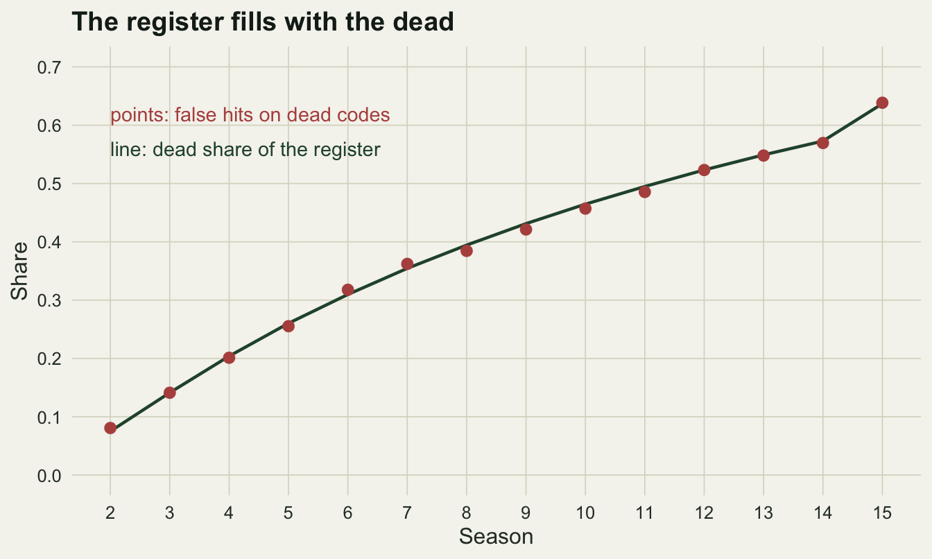
A false hit on a dead code is read by the CJS model as that bird still being alive. A single one extends the bird’s apparent life to the season of the hit, and the gap in between is absorbed as missed detections, so the model trades a little detection probability for survival. The measured result, with the resighting rate of 2 per live bird per season held fixed throughout:
Read correctly, the same birds give 0.8518, 0.8500 and 0.8498 at 5, 10 and 15 seasons, and the 95 per cent interval covers the true 0.85 in 94.5, 94.2 and 94.8 per cent of 400 studies. At a misread rate of 3 per cent, apparent survival reads 0.8599, 0.8610 and 0.8637. The part of that owed to misreads is the paired shift, the misread fit minus the correctly read fit of the same birds: +0.0081, +0.0110 and +0.0139, with standard errors of at most 0.0003, so it grows with every season. Against the true 0.85 the total bias is +0.0099, +0.0110 and +0.0137 (Monte Carlo standard errors of at most 0.0008); at 5 seasons that total includes an excess of +0.0018 (Monte Carlo standard error 0.0008) that the correctly read fits carry without any misreads. The detection estimate falls from 0.850 to 0.812, which is the other half of the trade. At a misread rate of 1 per cent and 15 seasons the paired shift is +0.0049 and coverage 81.5 per cent.
The biases are small, and that is exactly why they are dangerous. The sampling standard deviation of the estimate falls from 0.0169 at 5 seasons to 0.0075 at 10 and 0.0053 at 15, while the bias grows, so the interval covers the truth in 91.8, 69.5 and 28.5 per cent of studies (Monte Carlo standard errors up to 2.3 percentage points). The transients post already shows that an interval can be tight and wrong at one design; here the point is that the same study gets more wrong with every season of effort, because both the dead share of the register and the precision of the estimate increase with time. Coverage is driven jointly by the resighting rate, the misread rate and the study length (only the misread rate and the length were varied here), so these numbers belong to a resighting rate of 2; a better-watched scheme at the same misread rate is expected to lose coverage sooner.
lev_arm <- c("e = 0", "e = 0.01", "e = 0.03", "e = 0.03, two-sighting filter")
growth <- rbind(
  data.frame(K = ctrl_a$K, arm = lev_arm[1], phi = ctrl_a$phi0, cover = ctrl_a$cover0,
             g = which(tab_a$e == 0.03), filt = NA),
  data.frame(K = tab_a$K, arm = ifelse(tab_a$e == 0.01, lev_arm[2], lev_arm[3]),
             phi = tab_a$phi, cover = tab_a$cover, g = seq_len(nrow(tab_a)), filt = FALSE),
  data.frame(K = tab_a$K[tab_a$e == 0.03], arm = lev_arm[4],
             phi = tab_a$phi2[tab_a$e == 0.03], cover = tab_a$cover2[tab_a$e == 0.03],
             g = which(tab_a$e == 0.03), filt = TRUE))
growth$lo <- NA_real_; growth$hi <- NA_real_
for (i in seq_len(nrow(growth))) {
  col_phi <- if (is.na(growth$filt[i])) "clean.phi" else if (growth$filt[i]) "two.phi" else "all.phi"
  est <- runs_a[[growth$g[i]]]$fits[, col_phi]
  growth$lo[i] <- quantile(est, 0.025); growth$hi[i] <- quantile(est, 0.975)
}
growth$mcse <- sqrt(growth$cover * (1 - growth$cover) / n_study_a)
growth$arm <- factor(growth$arm, levels = lev_arm)
arm_cols <- setNames(c(te_ink, te_gold, te_rust, te_forest), lev_arm)
arm_shapes <- setNames(c(1, 16, 16, 17), lev_arm)
dodge <- position_dodge(width = 1.6)
p_phi <- ggplot(growth, aes(K, phi, colour = arm)) +
  geom_hline(yintercept = phi_true, linetype = 2, colour = te_body, linewidth = 0.3) +
  geom_errorbar(aes(ymin = lo, ymax = hi), width = 0, position = dodge, linewidth = 0.5) +
  geom_line(position = dodge, linewidth = 0.6) +
  geom_point(aes(shape = arm), position = dodge, size = 2.4, stroke = 1) +
  scale_colour_manual(values = arm_cols, name = NULL) +
  scale_shape_manual(values = arm_shapes, name = NULL) +
  scale_x_continuous(breaks = c(5, 10, 15)) +
  labs(x = "Seasons in the study", y = "Apparent survival",
       title = "Estimate") +
  theme_datasheet() + theme(legend.position = "bottom")
p_cov <- ggplot(growth, aes(K, cover, colour = arm)) +
  geom_hline(yintercept = 0.95, linetype = 2, colour = te_body, linewidth = 0.3) +
  geom_errorbar(aes(ymin = cover - 2 * mcse, ymax = pmin(1, cover + 2 * mcse)),
                width = 0, position = dodge, linewidth = 0.5) +
  geom_line(position = dodge, linewidth = 0.6) +
  geom_point(aes(shape = arm), position = dodge, size = 2.4, stroke = 1) +
  scale_colour_manual(values = arm_cols, name = NULL) +
  scale_shape_manual(values = arm_shapes, name = NULL) +
  scale_x_continuous(breaks = c(5, 10, 15)) +
  scale_y_continuous(limits = c(0, 1)) +
  labs(x = "Seasons in the study", y = "Coverage of the 95% interval",
       title = "Coverage") +
  theme_datasheet() + theme(legend.position = "bottom")
(p_phi | p_cov) +
  plot_layout(guides = "collect") +
  plot_annotation(theme = theme_datasheet()) &
  theme(legend.position = "bottom")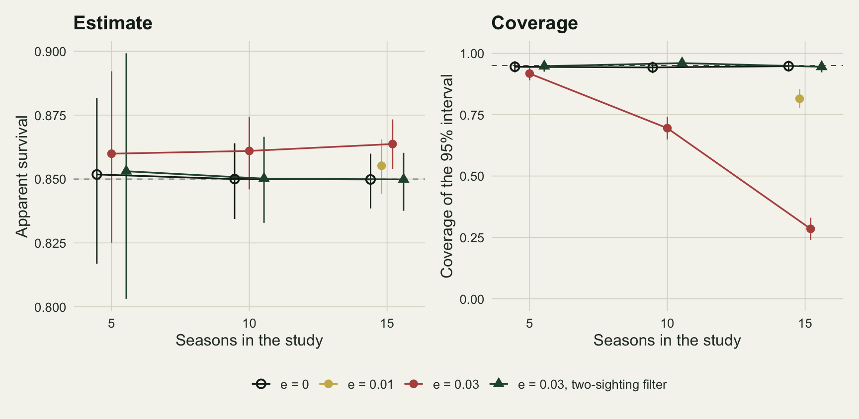
The two-sighting filter, when every bird is equally visible
The filter Tucker and colleagues evaluated counts a season for a bird only when its code was read at least twice. The logic is that a genuine bird is read repeatedly and a false hit is a one-off: two false hits rarely land on the same code in the same season, since there are only a handful of false hits spread over hundreds of codes. In the simulation where every bird has the same resighting rate, that logic holds.
b_sd_ratio_5 <- a5$sd2 / a5$sd
b_sd_ratio_15 <- a15$sd2 / a15$sd
print(round(tab_a[tab_a$e == 0.03, c("K", "phi2", "bias2", "sd2", "p2", "cover2")], 4))
K phi2 bias2 sd2 p2 cover2
1 5 0.8531 0.0031 0.0245 0.5820 0.9475
2 10 0.8502 0.0002 0.0086 0.5808 0.9600
3 15 0.8498 -0.0002 0.0059 0.5815 0.9450On the same simulated studies, the filter returns 0.8531, 0.8502 and 0.8498 at 5, 10 and 15 seasons, and the interval covers the truth in 94.8, 96.0 and 94.5 per cent of studies. The detection probability drops to 0.581, near the at-least-twice share computed above, and the price is precision: the standard deviation of the estimate is 1.45 times that of the unfiltered analysis at 5 seasons and 1.12 times at 15. The cost falls on the short studies, where the bias was smallest anyway. At 5 seasons the filtered estimate and the correctly read one both sit a little above 0.85, by 0.0031 and 0.0018, and the paired difference between them, filtered minus correctly read, is +0.0013 (standard error 0.0008). Most of the excess is carried by the correctly read fits, so it is there without misreads, which points to the small-sample behaviour of the five-season estimator rather than to the filter. Under homogeneity, then, the filter is a good trade, and this is the regime in which it looks like a general fix.
Unequal sightability turns the filter against you
Real birds are not equally visible. Some feed close to the sea wall where every observer walks, some use a distant creek, some carry a combination with a colour that fades. The third block gives each bird its own resighting rate from a gamma distribution with the same mean of 2 and a coefficient of variation of 0.5 or 1.0, and fits five models to every study: the constant CJS on all readings, the same with the filter, a two-class detection mixture of the kind Pledger, Pollock and Norris set out for the CJS model, the mixture with the filter, and the mixture plus a detection probability f for the dead state. Each study is fitted twice, once with its readings as the register join delivers them at a misread rate of 3 per cent and once as if every reading had been correct, and those paired control fits carry half of the argument. The five-model comparison runs on 50 studies per level because the mixture fits are slow; the two constant-model fits at a coefficient of variation of 0.5 are cheap, and are repeated on 1000 fresh studies.
n_study_c <- 50L
cv_levels <- c(0.5, 1)
model_lab <- c(const_all = "constant p, all readings",
               const_two = "constant p, two-sighting filter",
               mix_all = "two-class p, all readings",
               mix_two = "two-class p, two-sighting filter",
               mix_dead = "two-class p + dead-state f")
five_fits <- function(cnt) {
  h1 <- hist_of(cnt, 1); h2 <- hist_of(cnt, 2)
  md <- fit_hmm(h1, "twof")
  c(const_all = fit_marray(marray_of(h1))[["phi"]],
    const_two = fit_marray(marray_of(h2))[["phi"]],
    mix_all = fit_hmm(h1, "two")[["phi"]],
    mix_two = fit_hmm(h2, "two")[["phi"]],
    mix_dead = md[["phi"]], f_dead = md[["f"]])
}
set.seed(6203)
runs_c <- lapply(cv_levels, function(cv) {
  pairs <- replicate(n_study_c, {
    s <- sim_counts(10, 0.03, cv = cv)
    list(clean = five_fits(s$cnt0), misread = five_fits(s$cnt),
         dead = c(sum(s$fh$dead_seen), sum(s$fh$dead_codes)))
  }, simplify = FALSE)
  dead <- rowSums(sapply(pairs, function(z) z$dead))
  list(clean = t(sapply(pairs, function(z) z$clean[names(model_lab)])),
       misread = t(sapply(pairs, function(z) z$misread[names(model_lab)])),
       f_clean = mean(sapply(pairs, function(z) z$clean[["f_dead"]])),
       f_misread = mean(sapply(pairs, function(z) z$misread[["f_dead"]])),
       f_real = dead[1] / dead[2])
})
tab_c <- do.call(rbind, lapply(seq_along(cv_levels), function(g) {
  rc <- runs_c[[g]]
  rbind(data.frame(cv = cv_levels[g], e = 0, model = names(model_lab),
                   phi = colMeans(rc$clean), mcse = apply(rc$clean, 2, sd) / sqrt(n_study_c)),
        data.frame(cv = cv_levels[g], e = 0.03, model = names(model_lab),
                   phi = colMeans(rc$misread), mcse = apply(rc$misread, 2, sd) / sqrt(n_study_c)))
}))
shift_c <- do.call(rbind, lapply(seq_along(cv_levels), function(g) {
  dd <- runs_c[[g]]$misread - runs_c[[g]]$clean
  data.frame(cv = cv_levels[g], model = names(model_lab), shift = colMeans(dd),
             shift_se = apply(dd, 2, sd) / sqrt(n_study_c))
}))
print(reshape(tab_c[, c("cv", "e", "model", "phi")], idvar = c("cv", "e"),
              timevar = "model", direction = "wide"), digits = 4, row.names = FALSE)
cv e phi.const_all phi.const_two phi.mix_all phi.mix_two phi.mix_dead
0.5 0.00 0.8438 0.8224 0.8480 0.8424 0.8458
0.5 0.03 0.8551 0.8223 0.8623 0.8425 0.8470
1.0 0.00 0.8185 0.7632 0.8389 0.8355 0.8365
1.0 0.03 0.8336 0.7637 0.8569 0.8367 0.8426print(shift_c, digits = 3, row.names = FALSE) cv model shift shift_se
0.5 const_all 0.011291 0.000457
0.5 const_two -0.000125 0.000220
0.5 mix_all 0.014251 0.000592
0.5 mix_two 0.000186 0.000333
0.5 mix_dead 0.001189 0.000533
1.0 const_all 0.015073 0.000602
1.0 const_two 0.000404 0.000367
1.0 mix_all 0.017969 0.000874
1.0 mix_two 0.001183 0.000554
1.0 mix_dead 0.006106 0.000938get_c <- function(cv, e, model) tab_c$phi[tab_c$cv == cv & tab_c$e == e & tab_c$model == model]
get_shift <- function(cv, model) shift_c$shift[shift_c$cv == cv & shift_c$model == model]
get_shift_se <- function(cv, model) shift_c$shift_se[shift_c$cv == cv & shift_c$model == model]
mcse_c_max <- max(tab_c$mcse)
f_cost <- sapply(runs_c, function(rc) mean(rc$clean[, "mix_dead"] - rc$clean[, "mix_all"]))
f_cost_se <- sapply(runs_c, function(rc) sd(rc$clean[, "mix_dead"] - rc$clean[, "mix_all"]) /
sqrt(n_study_c))
f_c <- data.frame(cv = cv_levels, f_cost = f_cost, f_cost_se = f_cost_se,
f_hat_clean = sapply(runs_c, `[[`, "f_clean"),
f_hat_misread = sapply(runs_c, `[[`, "f_misread"),
f_real = sapply(runs_c, `[[`, "f_real"))
print(f_c, digits = 3, row.names = FALSE) cv f_cost f_cost_se f_hat_clean f_hat_misread f_real
0.5 -0.00216 0.000407 0.00194 0.0150 0.0149
1.0 -0.00243 0.000512 0.00161 0.0115 0.0145n_study_big <- 1000L
set.seed(8156)
big_c <- t(replicate(n_study_big, {
s <- sim_counts(10, 0.03, cv = 0.5)
c(all0 = fit_marray(marray_of(hist_of(s$cnt0, 1)))[["phi"]],
two0 = fit_marray(marray_of(hist_of(s$cnt0, 2)))[["phi"]],
all3 = fit_marray(marray_of(hist_of(s$cnt, 1)))[["phi"]],
two3 = fit_marray(marray_of(hist_of(s$cnt, 2)))[["phi"]])
}))
big_mean <- colMeans(big_c)
big_mcse <- apply(big_c, 2, sd) / sqrt(n_study_big)
big_rule_shift <- mean(big_c[, "two3"] - big_c[, "two0"])
big_rule_shift_se <- sd(big_c[, "two3"] - big_c[, "two0"]) / sqrt(n_study_big)
print(round(rbind(mean = big_mean, mcse = big_mcse), 4)) all0 two0 all3 two3
mean 0.8453 0.8246 0.8567 0.8245
mcse 0.0003 0.0003 0.0003 0.0003cv_p <- function(cv, rule, n_draw = 2e5) {
lam_i <- rgamma(n_draw, 1 / cv^2, scale = lam_mean * cv^2)
p_i <- if (rule == 1) 1 - exp(-lam_i) else 1 - exp(-lam_i) * (1 + lam_i)
sd(p_i) / mean(p_i)
}
set.seed(118)
cvp_one <- cv_p(0.5, 1); cvp_two <- cv_p(0.5, 2)In the five-model table the Monte Carlo standard errors of the means are at most 0.0023, and the paired shifts, misread fit minus correctly read fit on the same study, are known far more precisely than that.
Start with the constant model on 1000 studies at a coefficient of variation of 0.5. Read correctly, the birds give 0.8453: unequal sightability alone already pulls apparent survival down by 0.0047. With misreads the estimate is 0.8567, so the upward push of the false hits more than cancels that. The filter gives 0.8245, a bias of -0.0255 against +0.0067 without it: nearly four times larger and in the other direction (Monte Carlo standard errors 0.0003). The paired control says where it comes from. On the correctly read histories the filter gives 0.8246, and the paired shift from misreads under the filter is -0.0002 (standard error 0.0001). The filter does remove the misreads, to within 0.0002, even here. What it adds is a bias of its own, and that bias is there with no misreads at all.
The reason is in what the filter does to detection. A bird with resighting rate lam_i is detected with probability 1 - exp(-lam_i) under the usual scoring and 1 - exp(-lam_i) * (1 + lam_i) under the filter. For resighting rates with a coefficient of variation of 0.5, the per-bird detection probability has a coefficient of variation of 0.19 under the usual scoring and 0.43 under the filter. The filter spreads detection across birds, and a CJS model with one detection probability reads a bird that is persistently hard to see as a bird that died. That is the familiar downward bias of unmodelled heterogeneity in detection, and the filter more than doubles the heterogeneity it acts on.
A two-class detection mixture looks like the obvious answer to that, and on misread data it goes wrong in a new way. On the correctly read histories at a coefficient of variation of 0.5 it gives 0.8480 against the constant model’s 0.8438, so two classes take out part of the heterogeneity bias but not all of it. With misreads the mixture moves up by 0.0143, more than the constant model’s 0.0113: the low-detection class offers a home for dead birds that are “seen” now and then, and the model files them there as survivors that are hard to see. Adding the dead-state detection f to the mixture cuts the misread shift to 0.0012 (standard error 0.0005), and the fit reads 0.8470. Part of what remains against the truth is the price of f itself: on the correctly read histories, adding f moves the mixture from 0.8480 to 0.8458 (paired difference -0.0022, standard error 0.0004), because with no misreads at all f is still fitted at 0.0019 on average and absorbs some real late sightings of hard-to-see birds. The rest is heterogeneity that two classes miss.
At a coefficient of variation of 1.0 nothing here is clean, and the post does not call it a success. The mixture with f still moves up by 0.0061 with misreads, about a third of the plain mixture’s 0.0180, and reads 0.8426. On correctly read histories the plain mixture gives 0.8389 and adding f takes it to 0.8365 (paired difference -0.0024, standard error 0.0005); the plain mixture’s own gap from 0.85 shows how much heterogeneity two classes leave behind. The filtered constant model falls to 0.7637.
One row deserves a warning of its own. At a coefficient of variation of 1.0, the naive constant model is closer to the truth with misreads (0.8336) than without them (0.8185), because heterogeneity pulls the estimate down and misreads push it up. It is the open-population version of the cancelling pair in the identification errors post. A survival estimate that looks plausible can be two errors cancelling, and no amount of staring at the estimate will tell you which.
tab_c$model_f <- factor(model_lab[tab_c$model], levels = rev(model_lab))
tab_c$cv_f <- factor(sprintf("CV of resighting rate %.1f", tab_c$cv))
tab_c$e_f <- factor(ifelse(tab_c$e == 0, "no misreads", "3% misreads"),
                    levels = c("no misreads", "3% misreads"))
p_het <- ggplot(tab_c, aes(phi, model_f, colour = e_f)) +
  geom_vline(xintercept = phi_true, linetype = 2, colour = te_body, linewidth = 0.3) +
  geom_errorbar(aes(xmin = phi - 2 * mcse, xmax = phi + 2 * mcse), orientation = "y",
                width = 0, linewidth = 0.6,
                position = position_dodge(width = 0.5)) +
  geom_point(size = 2.6, position = position_dodge(width = 0.5)) +
  facet_wrap(~ cv_f, nrow = 1) +
  scale_x_continuous(breaks = seq(0.76, 0.86, 0.02)) +
  scale_colour_manual(values = c("no misreads" = te_body, "3% misreads" = te_rust),
                      name = NULL) +
  labs(x = "Mean apparent survival", y = NULL,
       title = "The filter's damage is there without misreads") +
  theme_datasheet() +
  theme(legend.position = "bottom",
        strip.text = element_text(colour = te_ink, face = "bold"))
p_het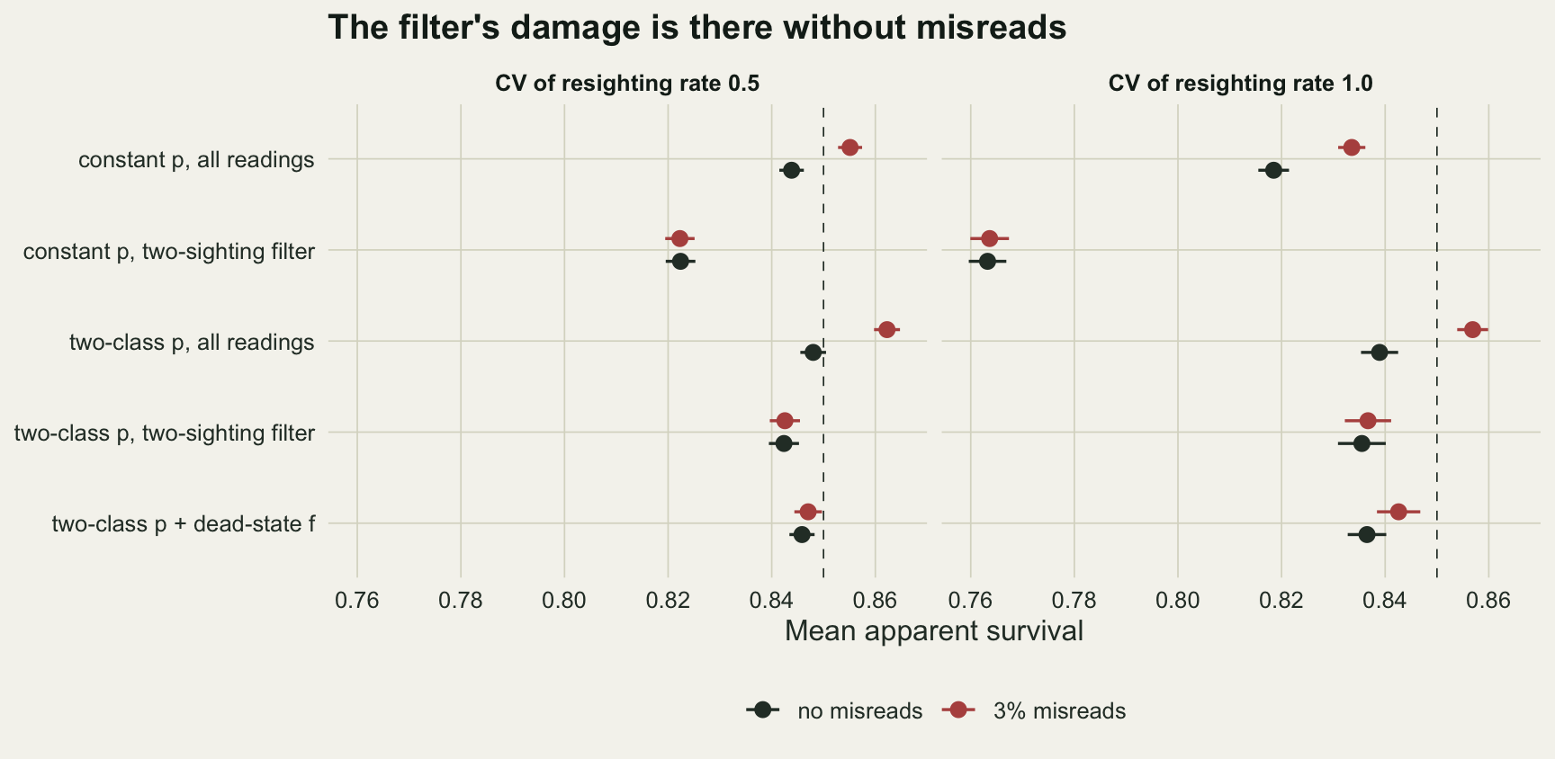
Modelling the false hit instead
The mixture with a dead-state detection probability is a small hidden Markov model. A bird is alive in one of two detection classes or dead; a live bird is detected with its class probability, and a dead bird whose code is still in the register is “detected” with probability f, the chance that at least one passing misread lands on it in a season. It needs no secondary sessions and no count of readings, only the binary season histories. The information that identifies f is the shape of the false record: a dead code’s false hits keep arriving at the same low rate for as long as the study runs, while a live bird’s detections, however sparse, stop when it dies, and while it lives they arrive at a class rate far above f. The fourth block asks whether the estimate from this model comes with an interval that covers, at a coefficient of variation of 0.5, 3 per cent misreads and ten seasons, and compares the fitted f with the realised rate at which dead codes were scored as seen.
n_study_d <- 100L
set.seed(7730)
fits_d <- vector("list", n_study_d); truth_d <- vector("list", n_study_d)
const_d <- vector("list", n_study_d)
for (i in seq_len(n_study_d)) {
  s <- sim_counts(10, 0.03, cv = 0.5)
  fits_d[[i]] <- fit_hmm(hist_of(s$cnt, 1), "twof", hess = TRUE)
  const_d[[i]] <- fit_marray(marray_of(hist_of(s$cnt, 1)))
  truth_d[[i]] <- s$fh
}
fits_d <- as.data.frame(do.call(rbind, fits_d))
const_d <- as.data.frame(do.call(rbind, const_d))
d_const_width <- median(const_d$hi - const_d$lo)
d_const_cover <- mean(covers(const_d$lo, const_d$hi))
ok_d <- is.finite(fits_d$lo) & is.finite(fits_d$hi)
n_fail_d <- sum(!ok_d)
d_phi <- mean(fits_d$phi)
d_mcse <- sd(fits_d$phi) / sqrt(n_study_d)
d_cover <- mean(covers(fits_d$lo[ok_d], fits_d$hi[ok_d]))
d_cover_mcse <- sqrt(d_cover * (1 - d_cover) / sum(ok_d))
d_width <- median(fits_d$hi[ok_d] - fits_d$lo[ok_d])
d_f <- mean(fits_d$f)
d_f_q <- quantile(fits_d$f, c(0.1, 0.9))
truth_d <- do.call(rbind, truth_d)
f_season <- aggregate(cbind(dead_seen, dead_codes, lam_alive, issued, n_reject) ~ t, truth_d, sum)
f_season$f_real <- f_season$dead_seen / f_season$dead_codes
f_season$f_expect <- 1 - exp(-0.03 * q_valid * f_season$lam_alive / f_season$issued)
f_season$f_reject <- 1 - exp(-f_season$n_reject * q_valid / (1 - q_valid) / f_season$issued)
f_pooled <- sum(f_season$dead_seen) / sum(f_season$dead_codes)
f_reject_pooled <- sum(f_season$f_reject * f_season$dead_codes) / sum(f_season$dead_codes)
print(round(f_season[, c("t", "dead_codes", "f_real", "f_expect", "f_reject")], 4))
t dead_codes f_real f_expect f_reject
1 2 1199 0.0092 0.0127 0.0156
2 3 3448 0.0148 0.0156 0.0149
3 4 6614 0.0157 0.0162 0.0155
4 5 10383 0.0153 0.0161 0.0163
5 6 14850 0.0147 0.0156 0.0163
6 7 19818 0.0154 0.0150 0.0146
7 8 25245 0.0138 0.0144 0.0139
8 9 31058 0.0137 0.0137 0.0135
9 10 37309 0.0142 0.0144 0.0141print(round(c(phi = d_phi, mcse = d_mcse, cover = d_cover, failed = n_fail_d,
width = d_width, const_width = d_const_width, const_cover = d_const_cover,
f_hat = d_f, f_pooled = f_pooled, f_reject = f_reject_pooled), 4)) phi mcse cover failed width const_width
0.8483 0.0009 0.9300 0.0000 0.0357 0.0302
const_cover f_hat f_pooled f_reject
0.8900 0.0141 0.0143 0.0145 Over 100 studies the model gives a mean apparent survival of 0.8483 (Monte Carlo standard error 0.0009), and its 95 per cent logit-Wald interval, from the numerical Hessian, covers 0.85 in 93 per cent of the 100 studies where the Hessian could be inverted (Monte Carlo standard error 2.6 percentage points; 0 failed). The median interval width is 0.036. The constant model fitted to the same studies gives a median width of 0.030 and covers 0.85 in 89 per cent of them, so the wider interval is the price of estimating a mixture and a false-detection rate from the same histories, and its coverage sits nearer to 95 per cent.
The fitted f averages 0.0141, with the central 80 per cent of studies between 0.0063 and 0.0233. The realised share of dead codes scored as seen, pooled over seasons and studies, is 0.0143. The model holds f constant, and the truth is not: the expected rate per dead code is e q lam N_alive / C, the misread flux of the live birds spread over every issued code, and over the nine resighting seasons the realised values run from 0.0092 to 0.0157, the expected ones from 0.0127 to 0.0162. Ringing continues in every season but the last here, so the live population and the register grow together and the ratio stays within that range, which is why a constant f is enough in this design; a scheme that stops ringing while it keeps resighting would see the ratio fall, and would need f to vary with time.
fits_d$rank <- rank(fits_d$phi, ties.method = "first")
fits_d$status <- ifelse(!ok_d, "no interval",
                        ifelse(covers(fits_d$lo, fits_d$hi), "covers 0.85", "misses 0.85"))
p_int <- ggplot(fits_d[ok_d, ], aes(y = rank)) +
  geom_vline(xintercept = phi_true, linetype = 2, colour = te_body, linewidth = 0.3) +
  geom_errorbar(aes(xmin = lo, xmax = hi, colour = status), orientation = "y",
                width = 0, linewidth = 0.45) +
  geom_point(aes(x = phi, colour = status), size = 0.9) +
  scale_colour_manual(values = c("covers 0.85" = te_forest, "misses 0.85" = te_rust),
                      name = NULL) +
  labs(x = "Apparent survival", y = "Study, sorted by estimate",
       title = "One interval per study") +
  theme_datasheet() + theme(legend.position = "bottom")
p_f <- ggplot(f_season, aes(t)) +
  annotate("rect", xmin = -Inf, xmax = Inf, ymin = d_f_q[1], ymax = d_f_q[2],
           fill = te_gold, alpha = 0.3) +
  geom_hline(yintercept = d_f, linetype = 2, colour = te_ink, linewidth = 0.4) +
  geom_line(aes(y = f_expect), colour = te_forest, linewidth = 0.7) +
  geom_point(aes(y = f_real), colour = te_rust, size = 2.4) +
  scale_x_continuous(breaks = 2:10) +
  scale_y_continuous(limits = c(0, NA)) +
  labs(x = "Season", y = "Dead codes scored as seen",
       title = "Fitted f against the truth") +
  theme_datasheet()
(p_int | p_f) + plot_annotation(theme = theme_datasheet())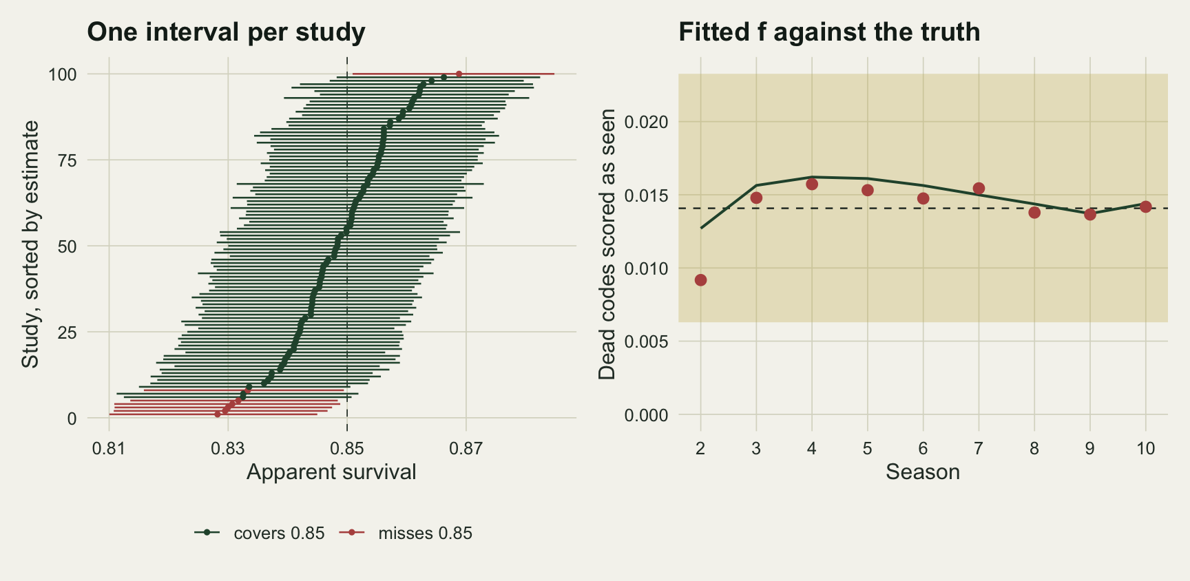
What to report
A CJS analysis built on resightings joined to a ring register should state how codes were checked against it and how many readings were rejected because they formed no issued code. That rejection count is the one piece of direct evidence about misreads that every scheme already has, and the harmful rate is the misread rate times the share of misreads that form a valid code, a share set by how densely the issued codes fill the space of possible combinations.
Report the study length beside any survival estimate from resightings. The bias measured here grows with the number of seasons, and a long-term series is where it is largest and where the interval is narrowest.
If a sighting filter is used, report the resighting rate distribution it was applied to, or at least the share of bird-seasons with exactly one reading, and fit the model with and without the filter. If the filtered estimate sits below the unfiltered one by more than misreads could explain, as it does here at a coefficient of variation of 0.5, the filter is acting on heterogeneity rather than on misreads.
If the data allow it, fit a model with a detection probability for the dead state and report the fitted f against the register rejection rate. The rejected readings estimate e (1 - q) times all readings, so the expected f in a season is about that season’s rejections times q / (1 - q), divided by the number of codes issued, with q roughly the share of possible combinations that has been issued. In the fourth block, where q is known to be 0.5, that rejection-based figure, pooled over dead codes as the realised rate is, comes to 0.0145 against a realised 0.0143. A scheme that double-reads a sample of birds estimates e directly. A near-zero f is reassuring; an f well above what the rejection count implies means something other than misreads is feeding the dead state, and on correctly read data f is not exactly zero either (the heterogeneity section above).
Honest limits
Every constant is fixed: 80 birds ringed a season, survival 0.85, a mean resighting rate of 2, and half of all misreads forming a valid code. The bias grows with the misread rate, the valid share and the resighting rate; only the first was varied here, giving a paired shift of +0.0049 at 1 per cent against +0.0139 at 3 per cent over 15 seasons, and none of the percentages above should be carried to another scheme without rerunning the code. In particular a share of valid codes other than 0.5 was not run, and alphanumeric flags, where most misreads form strings that were never issued, are likely to have a much smaller one.
Misreads here land uniformly on the register. Real misreads cluster: a combination is confused with its mirror image or with the one that differs by a faded colour, and some codes attract far more false hits than others. That would make f vary between dead birds, which the model here does not allow.
Survival and detection are constant in time. Tucker and colleagues and Rakhimberdiev and colleagues both report spurious declines in time-varying survival, a plausible consequence of the growing dead share of the register in a model that gives each year its own survival; this post fits only the constant model and does not measure the trend.
The coverage of the dead-state model was measured in one cell: a coefficient of variation of 0.5, ten seasons, 3 per cent misreads. It was not measured at 1.0, where the mean is already off and the fitted f falls to 0.0115 on misread data against a realised 0.0145 (at 0.5, in the same third-block studies, it is 0.0150 against 0.0149): the low-detection class and the dead state start to trade sightings. Nor was it measured at five seasons, where a dead code has few seasons in which to show its steady false-hit rate and f may be weakly identified. A mixture with more than two classes was not tried, and at a coefficient of variation of 1.0 it is the obvious next step.
The resighting counts are independent Poisson draws. Real readings of one bird on one day are correlated, because the same flock is scanned by several observers, and that makes a genuine bird read twice more likely than the Poisson says and a false hit read twice more likely too. How that changes the filter was not measured.
Finally, the model with f uses binary season histories only. The repair of Rakhimberdiev and colleagues uses the repeated readings within a season, which carry more information about which records are false, and when those data exist their model with secondary sessions is the stronger choice; the point here is that the ordinary season-level histories already contain enough to remove most of the misread shift at moderate heterogeneity, and about two thirds of it at a coefficient of variation of 1.0.
References
Tucker AM, McGowan CP, Robinson RA, Clark JA, Lyons JE, DeRose-Wilson A, du Feu R, Austin GE, Atkinson PW, Clark NA 2019 The Condor 121(1):duy017 (10.1093/condor/duy017)
Rakhimberdiev E, Karagicheva J, Saveliev A, Loonstra AHJ, Verhoeven MA, Hooijmeijer JCEW, Schaub M, Piersma T 2022 Methods in Ecology and Evolution 13(5):1106-1118 (10.1111/2041-210x.13825)
Pledger S, Pollock KH, Norris JL 2003 Biometrics 59(4):786-794 (10.1111/j.0006-341X.2003.00092.x)
Lebreton J-D, Burnham KP, Clobert J, Anderson DR 1992 Ecological Monographs 62(1):67-118 (10.2307/2937171)