library(ggplot2)

te_paper  <- "#f5f4ee"
te_ink    <- "#16241d"
te_body   <- "#2c3a31"
te_forest <- "#275139"
te_rust   <- "#b5534e"
te_gold   <- "#c9b458"
te_line   <- "#dad9ca"

theme_datasheet <- function() {
  theme_minimal(base_size = 12) +
    theme(plot.background  = element_rect(fill = te_paper, colour = NA),
          panel.background = element_rect(fill = te_paper, colour = NA),
          panel.grid.major = element_line(colour = te_line, linewidth = 0.3),
          panel.grid.minor = element_blank(),
          text             = element_text(colour = te_body),
          plot.title       = element_text(colour = te_ink, face = "bold"),
          plot.subtitle    = element_text(colour = te_body),
          axis.text        = element_text(colour = te_body))
}Identification errors in capture-recapture
R
capture-recapture
abundance
photo identification
simulation
ecology tutorial
A missed photo match inflates a capture-recapture estimate and a false match deflates it. Measuring in R why a cancelling pair still costs interval coverage.
A pond holds a population of great crested newts, and a survey team visits it on four nights. Every newt that comes out of a bottle trap is photographed belly up, because the pattern of black blotches on the orange belly is unique to the animal, and then released. After the season someone sits down with several hundred photographs and a growing catalogue, and for each new photograph decides one of two things: this is an animal already in the catalogue, or this is a new one. The capture histories, and so the abundance estimate, are nothing more than the record of those decisions.
The decision can go wrong in two ways, and they are not mirror images. A missed match happens when the photograph shows a newt that is already catalogued and the reader does not find it: the photograph opens a new entry, and one animal is now two. A false match happens when the photograph shows a newt that has never been caught and the reader files it under a look-alike: two animals are now one.
The basic arithmetic of closed populations is on this site already. Closed-population capture-recapture in R fits Lincoln-Petersen, Schnabel and the model M0 likelihood on histories in which every animal is recorded under its own identity. Capture heterogeneity: Mt, Mb and Mh measures what happens when M0 is fitted to animals that do not behave the way it assumes, and it finds two failures that push the estimate in opposite directions. Its honest limits add, without measuring it, that such opposite biases can cancel in the estimate while the interval goes wrong. This post measures exactly that possibility for a different pair of failures: the animals behave perfectly, and the catalogue does not.
Misidentification is also on the site at a different level. False positives in occupancy models deals with a species recorded at a site where it is absent, where a small error rate only ever pushes occupancy up. There the object that is misread is a species; here it is an individual, and the two directions of error are what make the problem harder to see.
The post does four things. It sets out the two error processes and the M0 likelihood, and checks the fit on clean histories. It measures how far each error moves the estimate. It searches for a pair of error rates that cancels in the point estimate, on a fixed grid, and measures what the cancelling pair does to the spread and the interval. Finally it asks whether the capture frequency table, the only diagnostic an analyst has, can see any of it.
Two ways to read a photograph wrongly
The population is closed and M0 is true of the animals: 200 newts, four nights, and a probability of 0.30 that a given newt is caught and photographed on a given night, the same for every animal and every night. All of the error lives in the catalogue.
The catalogue is built night by night, in the order a reader would build it. On each night every photograph belongs to one of two kinds. A photograph of an animal that already has an entry can suffer a missed match, with probability e_miss; when it does, it opens a new entry holding that single capture, and the animal’s own entry loses the capture. Later photographs of the same animal are compared against the catalogue again and usually find the original entry, so the new entry stays a one-capture ghost. A photograph of an animal that has no entry yet can suffer a false match, with probability e_false, as long as the catalogue is not empty; it is then filed under an existing entry chosen at random, and the animal stays filed there on every later night, because whatever made it look like that entry does not go away. When the animal and its look-alike are both caught on the same night, the entry records a single capture for that night, as a catalogue would.
The two rates are therefore rates per photograph of the kind that can suffer the error, not per animal. Three streams of uniform random numbers are drawn once per simulated study and shared by every error setting, so that each setting reads the same animals and the same photographs; only the thresholds change.
n_true <- 200      # newts in the pond
n_occ  <- 4        # survey nights
p_cap  <- 0.30     # probability a newt is caught and photographed on a night

build_catalogue <- function(caps, u_miss, u_false, u_pick, e_miss, e_false) {
  n_anim  <- nrow(caps)
  cat_id  <- rep(NA_integer_, n_anim)   # catalogue entry each animal is filed under
  next_id <- 1L
  rec_id  <- integer(0); rec_occ <- integer(0)
  n_ghost <- 0L; n_merge <- 0L
  for (occ in seq_len(n_occ)) {
    caught <- which(caps[, occ] == 1)
    known  <- caught[!is.na(cat_id[caught])]
    fresh  <- caught[is.na(cat_id[caught])]
    n_cat  <- next_id - 1L
    # false match: a new animal is filed under an existing entry, for good
    merged <- if (n_cat > 0) fresh[u_false[fresh, occ] < e_false] else integer(0)
    cat_id[merged] <- pmax(1L, ceiling(u_pick[merged, occ] * n_cat))
    filed <- fresh[!fresh %in% merged]
    cat_id[filed] <- next_id + seq_along(filed) - 1L
    next_id <- next_id + length(filed)
    # missed match: a known animal's photograph opens a new entry of its own
    missed <- known[u_miss[known, occ] < e_miss]
    ghost  <- next_id + seq_along(missed) - 1L
    next_id <- next_id + length(missed)
    matched <- known[!known %in% missed]
    rec_id  <- c(rec_id, cat_id[merged], cat_id[filed], ghost, cat_id[matched])
    rec_occ <- c(rec_occ, rep(occ, length(caught)))
    n_ghost <- n_ghost + length(missed); n_merge <- n_merge + length(merged)
  }
  hist_mat <- matrix(0L, next_id - 1L, n_occ)
  hist_mat[cbind(rec_id, rec_occ)] <- 1L
  list(hist = hist_mat, n_ghost = n_ghost, n_merge = n_merge)
}
The M0 likelihood, checked on clean histories
The estimator is the closed population model M0 of Otis and colleagues, fitted by maximum likelihood. With M distinct entries in the catalogue and n captures in total over K nights, the likelihood in N and p is proportional to N! / (N - M)! times p^n (1 - p)^(KN - n). For fixed N the best p is n / (KN), so the fit is a one dimensional maximisation of the profile over N, treated as continuous through the log gamma function. The interval is the profile likelihood interval: every N whose profile log likelihood lies within half of the 95 per cent chi squared quantile of the maximum.
The fit also returns the one diagnostic this post leans on later. Conditional on the M entries seen, the number of captures per entry follows a binomial distribution truncated at zero, with the fitted p. The observed counts caught once, twice, and three or more times are compared with that expectation by a Pearson chi squared statistic. Three cells, less one for the fixed total and one for the fitted p, leave one degree of freedom.
m0_profile <- function(N, m_seen, n_caps) {
  p <- n_caps / (n_occ * N)
  lgamma(N + 1) - lgamma(N - m_seen + 1) +
    n_caps * log(p) + (n_occ * N - n_caps) * log(1 - p)
}

fit_m0 <- function(hist_mat) {
  m_seen <- nrow(hist_mat); n_caps <- sum(hist_mat)
  top  <- 20 * m_seen
  opt  <- optimize(m0_profile, c(m_seen, top), m_seen = m_seen, n_caps = n_caps,
                   maximum = TRUE, tol = 1e-4)
  cut_ll <- opt$objective - qchisq(0.95, 1) / 2
  prof_gap <- function(N) m0_profile(N, m_seen, n_caps) - cut_ll
  lo <- if (prof_gap(m_seen) >= 0) m_seen else uniroot(prof_gap, c(m_seen, opt$maximum))$root
  hi <- uniroot(prof_gap, c(opt$maximum, top))$root
  p_hat <- n_caps / (n_occ * opt$maximum)
  f_j   <- tabulate(rowSums(hist_mat), n_occ)
  cell_p <- dbinom(seq_len(n_occ), n_occ, p_hat)
  cell_p <- cell_p / sum(cell_p)
  obs_c <- c(f_j[1], f_j[2], sum(f_j[3:n_occ]))
  exp_c <- m_seen * c(cell_p[1], cell_p[2], sum(cell_p[3:n_occ]))
  resid <- (obs_c - exp_c) / sqrt(exp_c)
  c(N_hat = opt$maximum, lo = lo, hi = hi, p_hat = p_hat, m_seen = m_seen,
    f1 = f_j[1], f2 = f_j[2], f3 = f_j[3], f4 = f_j[4],
    r1 = resid[1], r2 = resid[2], r3 = resid[3], chi = sum(resid^2))
}

one_study <- function(n_anim, rate_pairs) {
  caps <- matrix(rbinom(n_anim * n_occ, 1, p_cap), n_anim, n_occ)
  u_m  <- matrix(runif(n_anim * n_occ), n_anim)
  u_f  <- matrix(runif(n_anim * n_occ), n_anim)
  u_p  <- matrix(runif(n_anim * n_occ), n_anim)
  out <- apply(rate_pairs, 1, function(rr) {
    cat_run <- build_catalogue(caps, u_m, u_f, u_p, rr[1], rr[2])
    c(fit_m0(cat_run$hist), ghosts = cat_run$n_ghost, merges = cat_run$n_merge)
  })
  t(out)
}

run_studies <- function(n_anim, rate_pairs, n_rep) {
  simplify2array(lapply(seq_len(n_rep), function(i) one_study(n_anim, rate_pairs)))
}set.seed(307)
one_caps <- matrix(rbinom(n_true * n_occ, 1, p_cap), n_true, n_occ)
one_hist <- one_caps[rowSums(one_caps) > 0, ]
one_fit <- fit_m0(one_hist)
int_grid <- nrow(one_hist):(nrow(one_hist) + 400)
int_ll <- m0_profile(int_grid, nrow(one_hist), sum(one_hist))
int_best <- int_grid[which.max(int_ll)]
n_clean <- 2000
set.seed(3071)
clean_runs <- run_studies(n_true, rbind(c(0, 0)), n_clean)[1, , ]
clean_mean <- mean(clean_runs["N_hat", ])
clean_cov <- mean(clean_runs["lo", ] <= n_true & clean_runs["hi", ] >= n_true)
clean_rej <- mean(clean_runs["chi", ] > qchisq(0.95, 1))
clean_seen <- mean(clean_runs["m_seen", ])Two checks come before any error is added. On one simulated study with 149 newts seen, the continuous maximiser returns 204.04, and a brute force search over the integers from the number seen upwards puts the maximum at 204, so the optimiser is finding the peak of the likelihood as written.
Over 2000 clean studies the mean estimate is 200.1 against a true 200, with 152.1 newts seen on average. The profile interval covers the truth in 95.0 per cent of studies and the goodness of fit test rejects in 5.3 per cent, both at their nominal values to within Monte Carlo error. Whatever goes wrong below is caused by the catalogue.
Each error pushes the estimate its own way
The mechanism is visible in the two summary statistics M0 uses. A missed match adds an entry without adding a capture, so there are fewer captures per entry; the fitted p goes down and the estimated number never seen goes up. A false match removes an entry, and moves its captures onto another one, so there are more captures per entry; p goes up and the estimate goes down.
The measurement runs each error alone at eight rates from 2.5 to 20 per cent in steps of 2.5, and both together at equal rates, in 1000 studies of 200 newts and 400 studies of 2000 animals. The large studies are used in the last section.
err_rates <- seq(0.025, 0.20, by = 0.025)
grid_pairs <- rbind(c(0, 0),
                    cbind(err_rates, 0),
                    cbind(0, err_rates),
                    cbind(err_rates, err_rates))
grid_kind <- c("none", rep(c("missed matches only", "false matches only", "both at the same rate"),
                           each = length(err_rates)))
grid_rate <- c(0, rep(err_rates, 3))
n_rep_small <- 1000
n_rep_large <- 400
n_large     <- 2000

set.seed(30711)
grid_small <- run_studies(n_true, grid_pairs, n_rep_small)
set.seed(30712)
grid_large <- run_studies(n_large, grid_pairs, n_rep_large)

summarise_grid <- function(arr, n_anim, n_rep) {
  rel  <- arr[, "N_hat", ] / n_anim
  rej  <- arr[, "chi", ] > qchisq(0.95, 1)
  data.frame(kind = grid_kind, rate = grid_rate, n_anim = n_anim,
             rel_mean = rowMeans(rel),
             rel_se   = apply(rel, 1, sd) / sqrt(n_rep),
             reject   = rowMeans(rej),
             reject_se = sqrt(rowMeans(rej) * (1 - rowMeans(rej)) / n_rep),
             ghosts = rowMeans(arr[, "ghosts", ]),
             merges = rowMeans(arr[, "merges", ]))
}
sum_small <- summarise_grid(grid_small, n_true, n_rep_small)
sum_large <- summarise_grid(grid_large, n_large, n_rep_large)

pick <- function(tab, kind, rate) tab[tab$kind == kind & abs(tab$rate - rate) < 1e-9, ]
miss05  <- pick(sum_small, "missed matches only", 0.05)
false05 <- pick(sum_small, "false matches only", 0.05)
miss10  <- pick(sum_small, "missed matches only", 0.10)
false10 <- pick(sum_small, "false matches only", 0.10)
miss20  <- pick(sum_small, "missed matches only", 0.20)
false20 <- pick(sum_small, "false matches only", 0.20)
# photographs exposed to each error, expected from the design constants
first_caps   <- n_true * (1 - (1 - p_cap)^n_occ)   # animals caught at least once
recap_photos <- n_true * n_occ * p_cap - first_caps  # can suffer a missed match
late_first   <- first_caps - n_true * p_cap          # first captures after night one

ghost_mult <- (miss05$rel_mean - 1) * n_true / miss05$ghosts
merge_mult <- (1 - false05$rel_mean) * n_true / false05$merges
miss_curve  <- sum_small[sum_small$kind %in% c("none", "missed matches only"), ]
false_curve <- sum_small[sum_small$kind %in% c("none", "false matches only"), ]
miss_steps  <- 100 * diff(miss_curve$rel_mean)
false_steps <- 100 * diff(false_curve$rel_mean)
both20_small <- pick(sum_small, "both at the same rate", 0.20)
At a missed match rate of five per cent the catalogue gains 4.3 ghost entries per study on average, and the mean estimate is 213.4, 6.7 per cent too high. At a false match rate of five per cent 4.5 newts disappear into other entries and the estimate is 189.5, 5.3 per cent too low. Each ghost is worth 3.1 animals of bias and each merge 2.3, because the error changes both the count of entries and the fitted capture probability that scales it up.
The size of these biases depends on how many photographs are exposed to each error, and that depends on the capture probability and the number of nights. In this design a study has on average 88 recapture photographs, which are the ones that can suffer a missed match, and 92 first captures after the first night, which are the ones that can suffer a false match. A bias quoted per error rate without the design attached is therefore not a property of misidentification.
The missed match curve bends upwards and the false match curve very slightly flattens: each step of 2.5 points adds between 3.2 and 4.8 per cent to the missed match bias, and takes between 2.2 and 2.8 per cent off the estimate for false matches. At twenty per cent missed matches the estimate is 31.8 per cent high; at twenty per cent false matches it is 19.7 per cent low.
bias_df <- sum_small[sum_small$kind != "both at the same rate", ]
bias_df <- rbind(transform(bias_df[bias_df$kind == "none", ], kind = "missed matches only"),
                 transform(bias_df[bias_df$kind == "none", ], kind = "false matches only"),
                 bias_df[bias_df$kind != "none", ])
ggplot(bias_df, aes(100 * rate, n_true * rel_mean, colour = kind)) +
  geom_hline(yintercept = n_true, linetype = "dashed", colour = te_body, linewidth = 0.5) +
  geom_errorbar(aes(ymin = n_true * (rel_mean - 2 * rel_se),
                    ymax = n_true * (rel_mean + 2 * rel_se)), width = 0.6, linewidth = 0.5) +
  geom_line(linewidth = 0.9) +
  geom_point(size = 2.2) +
  scale_colour_manual(values = c("missed matches only" = te_rust,
                                 "false matches only" = te_forest), name = NULL) +
  labs(x = "error rate (per cent of the photographs that can suffer it)",
       y = "mean M0 estimate of N",
       title = "Missed matches inflate N, false matches deflate it",
       subtitle = "200 newts, 4 nights, capture probability 0.30; bars are two Monte Carlo SE") +
  theme_datasheet() +
  theme(legend.position = "bottom")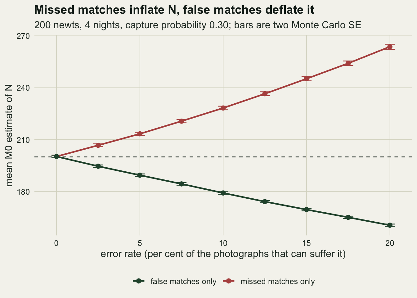
A pair of errors that cancels
Because the two errors push in opposite directions, some pair of rates must leave the mean estimate where it would have been without error. The pair was found by a fixed search, not by trying rates until one looked right; pilot runs with other seeds had already tried equal rates of five per cent, which came close to cancelling, and had already run this same search on this same grid, which is why the grid is centred there; none of the pilot numbers is used here. The missed match rate is held at five per cent, the value used above. The false match rate runs from zero to ten per cent in steps of one point. At each step the shift is the mean difference between the estimate with errors and the estimate from the same study read without error, over 2000 studies, and the cancelling rate is the zero crossing of that curve by linear interpolation. The rate is then used, unchanged, in a fresh set of 4000 studies with a new seed, and every number about the cancelling pair below comes from that second run.
miss_fixed <- 0.05
false_grid <- seq(0, 0.10, by = 0.01)
cancel_pairs <- rbind(c(0, 0), cbind(miss_fixed, false_grid))
n_rep_search <- 2000
set.seed(30713)
search_runs <- run_studies(n_true, cancel_pairs, n_rep_search)
shift_rep  <- sweep(search_runs[-1, "N_hat", ], 2, search_runs[1, "N_hat", ])
shift_mean <- rowMeans(shift_rep)
shift_se   <- apply(shift_rep, 1, sd) / sqrt(n_rep_search)
shift_monotone <- all(diff(shift_mean) < 0)
false_cancel <- approx(shift_mean, false_grid, xout = 0)$y

n_rep_confirm <- 4000
set.seed(30714)
confirm_runs <- run_studies(n_true, rbind(c(0, 0), c(miss_fixed, false_cancel)), n_rep_confirm)
conf_stats <- function(r, n_anim) {
  c(mean = mean(r["N_hat", ]), sd = sd(r["N_hat", ]),
    width = mean(r["hi", ] - r["lo", ]),
    cover = mean(r["lo", ] <= n_anim & r["hi", ] >= n_anim),
    f1 = mean(r["f1", ]), f2 = mean(r["f2", ]), f3 = mean(r["f3", ]), f4 = mean(r["f4", ]),
    seen = mean(r["m_seen", ]), reject = mean(r["chi", ] > qchisq(0.95, 1)),
    ghosts = mean(r["ghosts", ]), merges = mean(r["merges", ]))
}
conf_clean <- conf_stats(confirm_runs[1, , ], n_true)
conf_pair  <- conf_stats(confirm_runs[2, , ], n_true)
conf_shift <- confirm_runs[2, "N_hat", ] - confirm_runs[1, "N_hat", ]
conf_shift_mean <- mean(conf_shift)
conf_shift_se   <- sd(conf_shift) / sqrt(n_rep_confirm)
cover_se <- sqrt(conf_pair["cover"] * (1 - conf_pair["cover"]) / n_rep_confirm)
sd_ratio <- conf_pair["sd"] / conf_clean["sd"]
# F test style ratio of variances has its own sampling error; a bootstrap gives it
set.seed(30715)
sd_ratio_boot <- replicate(500, {
  idx <- sample.int(n_rep_confirm, replace = TRUE)
  sd(confirm_runs[2, "N_hat", idx]) / sd(confirm_runs[1, "N_hat", idx])
})
sd_ratio_ci <- quantile(sd_ratio_boot, c(0.025, 0.975))
shift_r2 <- summary(lm(conf_shift ~ confirm_runs[2, "ghosts", ] + confirm_runs[2, "merges", ]))$r.squared
cancel_df <- data.frame(rate = false_grid, shift = shift_mean, se = shift_se)
ggplot(cancel_df, aes(100 * rate, shift)) +
geom_hline(yintercept = 0, linetype = "dashed", colour = te_body, linewidth = 0.5) +
geom_vline(xintercept = 100 * false_cancel, colour = te_gold, linewidth = 0.8) +
geom_errorbar(aes(ymin = shift - 2 * se, ymax = shift + 2 * se), width = 0.3,
colour = te_forest, linewidth = 0.5) +
geom_line(colour = te_forest, linewidth = 0.9) +
geom_point(colour = te_forest, size = 2.2) +
annotate("text", x = 100 * false_cancel + 0.2, y = max(shift_mean) * 0.85,
label = paste0("zero crossing at ", sprintf("%.2f", 100 * false_cancel), " per cent"),
hjust = 0, colour = te_ink, size = 3.6) +
scale_x_continuous(breaks = seq(0, 10, by = 2)) +
labs(x = "false match rate (per cent), missed match rate held at 5 per cent",
y = "mean shift in the M0 estimate",
title = "The search for a cancelling pair",
subtitle = "shift against the same studies read without error; bars are two Monte Carlo SE") +
theme_datasheet()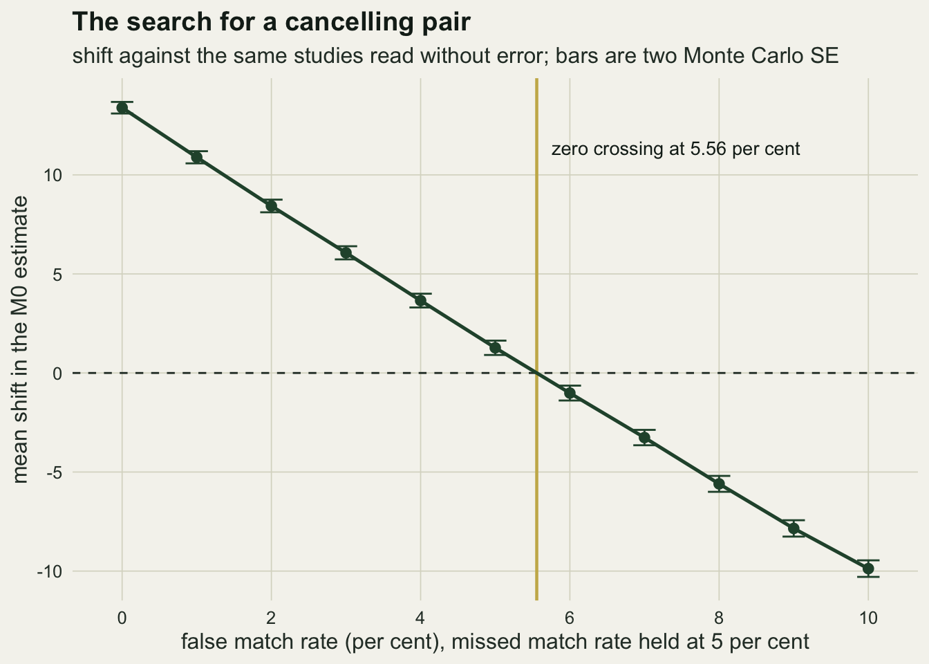
The shift falls steadily from 13.4 animals with no false matches to -9.9 at ten per cent, and crosses zero at a false match rate of 5.56 per cent. The cancelling pair is close to equal rates in this design, although each ghost moves the estimate more than each merge (3.1 animals against 2.3). Part of the reason is that the photographs exposed to each error happen to be similar in number, 88 against 92 per study; that coincidence depends on the capture probability and the number of nights, and nothing about misidentification makes it carry to another design.
In the confirmation run the mean shift is -0.01 animals with a Monte Carlo standard error of 0.13, and the mean estimates with and without errors are 200.0 and 200.0. The cancellation holds out of sample. A reader of the mean estimate has no way to tell the two catalogues apart.
The estimates do not have the same spread. The standard deviation of the estimate across studies is 11.90 for the clean catalogue and 13.77 for the catalogue with both errors, a ratio of 1.157 with a bootstrap interval from 1.133 to 1.179. The number of ghosts and merges in each study explains 96 per cent of the variance of the shift, so the extra spread comes from the study-to-study randomness in how many errors happen, a variation M0 has no term for. The model does not see it: the mean width of the profile interval is 47.9 with errors against 47.2 without. With the spread wider and the interval almost unchanged, coverage drops from 95.0 to 91.1 per cent, with a Monte Carlo standard error of 0.4 points.
The frequency table has moved too, although the total number of entries has barely changed (151.3 against 152.1). Entries caught once go from 82.4 to 83.9, entries caught twice fall from 52.9 to 50.2, and entries caught on all four nights go from 1.57 to 2.02. The ghosts fill the first class and the merged look-alikes the last. Whether a test can see that is the next question.
The singleton fingerprint is not where it was expected
The obvious candidate for a fingerprint of missed matches is an excess of animals caught once, since every ghost is one. The trouble is that M0 is fitted to the same table. A catalogue full of ghosts has a low capture rate per entry, the fitted p drops, and a low p predicts many animals caught once. The model answers the excess by adjusting the parameter the excess changed, and only what that adjustment cannot absorb is left for a diagnostic to find.
To see what is left after the fit, the next run uses studies of 2000 animals, ten times the pond, so that small systematic departures are not buried in noise, and averages the standardised residuals of the three frequency cells over 1000 studies.
finger_pairs <- rbind(c(0, 0), c(miss_fixed, 0), c(0, miss_fixed), c(miss_fixed, false_cancel))
finger_lab <- c("no errors", "missed matches, 5 per cent", "false matches, 5 per cent",
                "the cancelling pair")
n_rep_finger <- 1000
set.seed(30716)
finger_runs <- run_studies(n_large, finger_pairs, n_rep_finger)
finger_reject <- rowMeans(finger_runs[, "chi", ] > qchisq(0.95, 1))
finger_cover  <- rowMeans(finger_runs[, "lo", ] <= n_large & finger_runs[, "hi", ] >= n_large)
finger_rel    <- rowMeans(finger_runs[, "N_hat", ]) / n_large
finger_resid  <- sapply(c("r1", "r2", "r3"), function(cc) rowMeans(finger_runs[, cc, ]))
finger_se_rej <- sqrt(finger_reject * (1 - finger_reject) / n_rep_finger)
fp_df <- data.frame(scenario = factor(rep(finger_lab, 3), levels = finger_lab),
cell = factor(rep(c("caught once", "caught twice", "three or more"),
each = length(finger_lab)),
levels = c("caught once", "caught twice", "three or more")),
resid = as.vector(finger_resid))
ggplot(fp_df, aes(cell, resid, fill = scenario)) +
geom_hline(yintercept = 0, colour = te_body, linewidth = 0.4) +
geom_col(position = position_dodge(width = 0.8), width = 0.75) +
scale_fill_manual(values = c(te_line, te_rust, te_forest, te_gold), name = NULL) +
guides(fill = guide_legend(nrow = 2)) +
labs(x = "capture frequency class", y = "mean standardised residual",
title = "What the frequency table shows after M0 has adjusted p",
subtitle = "2000 animals, 4 nights; residual of observed against fitted, averaged over studies") +
theme_datasheet() +
theme(legend.position = "bottom")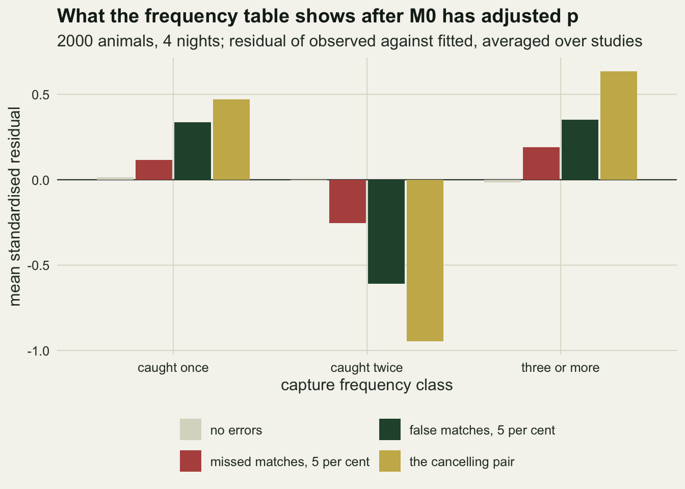
The residuals have the same shape in all three error scenarios: too many entries caught once, too few caught twice, too many caught three or more times. For missed matches alone the mean residual of the caught once class is 0.12; for false matches alone it is 0.34, larger, even though false matches remove animals rather than adding ghosts. A merged look-alike usually carries more captures than a single animal would, the fitted p rises to match it, and the singletons that are left then look too many for that p. The excess of singletons is not a fingerprint of missed matches; it is a fingerprint of a frequency distribution wider than a binomial, and both errors make one. The cancelling pair has the largest residual in every class in absolute value, 0.47 for the caught once class, because it widens the distribution from both ends at once.
The goodness of fit test is the formal version of that picture, and its rejection rate across the whole error grid is the next figure.
pow_df <- rbind(sum_small, sum_large)
pow_df <- pow_df[pow_df$kind != "none", ]
zero_rows <- rbind(sum_small[1, ], sum_large[1, ])
pow_df <- rbind(pow_df,
                do.call(rbind, lapply(unique(pow_df$kind), function(kk) transform(zero_rows, kind = kk))))
pow_df$study <- factor(ifelse(pow_df$n_anim == n_true, "200 animals", "2000 animals"),
                       levels = c("200 animals", "2000 animals"))
pow_df <- pow_df[order(pow_df$study, pow_df$kind, pow_df$rate), ]
ggplot(pow_df, aes(100 * rate, reject, colour = kind)) +
  geom_hline(yintercept = 0.05, linetype = "dashed", colour = te_body, linewidth = 0.5) +
  geom_line(linewidth = 0.9) +
  geom_point(size = 1.9) +
  facet_wrap(~ study) +
  scale_colour_manual(values = c("missed matches only" = te_rust,
                                 "false matches only" = te_forest,
                                 "both at the same rate" = te_gold), name = NULL) +
  scale_y_continuous(limits = c(0, 1)) +
  labs(x = "error rate (per cent)", y = "rejection rate of the M0 goodness of fit test",
       title = "The goodness of fit test barely sees missed matches",
       subtitle = "chi squared on caught once, twice, three or more; 5 per cent level dashed") +
  theme_datasheet() +
  theme(legend.position = "bottom",
        strip.text = element_text(colour = te_ink, face = "bold"),
        panel.spacing = unit(1.2, "lines"))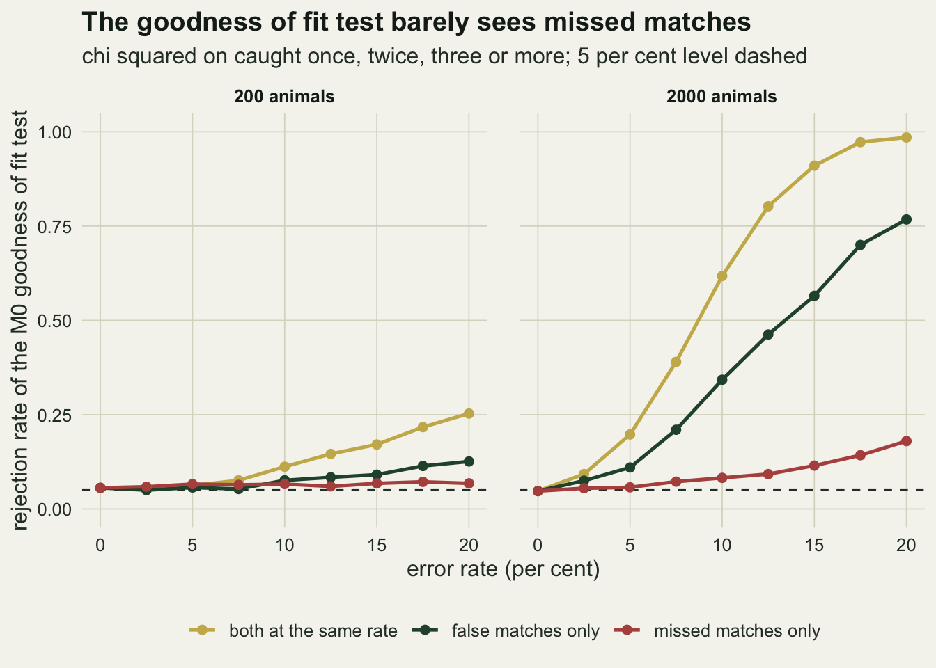
In the pond of 200 newts the test is close to blind to missed matches and weak against the rest. At twenty per cent missed matches it rejects in 6.8 per cent of studies, while the estimate is 32 per cent high; at twenty per cent false matches it rejects in 12.6 per cent; with both at twenty per cent, in 25.3 per cent.
With 2000 animals the test starts to work, and it works in the reverse of the order the singleton argument suggests. For the three five per cent scenarios of the fingerprint run it rejects in 6.2 per cent of studies with missed matches, 13.2 per cent with false matches and 23.2 per cent with the cancelling pair, against 5.1 per cent without error (Monte Carlo standard errors at most 1.3 points). The error that inflates abundance, the one most analysts worry about, is the one the table hides best, and the cancelling pair, which leaves the mean estimate untouched, is the one it shows most clearly. Meanwhile the interval for the large study covers the truth in 9.7 per cent of studies with missed matches alone and 16.2 per cent with false matches alone, because with ten times the animals the interval is narrow and the bias is not.
What to report
State the matching protocol and put a number on each error rate. The frequency table cannot supply them: in a study of ordinary size the goodness of fit test did not tell a catalogue with one ghost in five recaptures from a clean one. The measurement that does is a re-match of a subsample of photographs against animals whose identity is known independently (a second, permanent mark, or a reference set resolved by several readers), which gives the missed and the false match rates separately; a second reader alone gives only the rate of disagreement.
Report the two rates separately, not as one misidentification rate. They bias abundance in opposite directions, so a single combined rate says nothing about the sign of the error, and a small net bias is not evidence that both rates are small.
If both errors are plausible, do not treat an estimate that agrees with an independent count as proof that the catalogue is clean. The cancelling pair above matched the error-free mean to within Monte Carlo error while its interval covered the truth in 91.1 per cent of studies instead of 95.
Give the full capture frequency table and the number of recaptures: with a missed match rate from a calibration exercise, the recaptures give the expected number of ghosts, and the table lets a reader refit.
Honest limits
The error model is one of several reasonable ones. A missed match here creates a single ghost, because the animal’s later photographs are compared against its original entry. With marks that change over time, the case Yoshizaki and colleagues set out for photographic identification, the new entry would be the one later photographs match, and one history would split into two longer pieces rather than losing one capture to a singleton. Nothing above measures that version. The misidentification model of Link and colleagues lets any capture, including the first, produce a ghost, so its rate is per photograph of any kind and is not the same number as the missed match rate here.
The false match here is permanent and falls on an entry chosen at random. A real reader confuses animals that look alike, so the confusions cluster on a few pattern types, and some false matches are later noticed and undone. A third error, filing a photograph of a catalogued animal under a different catalogued animal, is left out altogether; since M0 uses only the number of entries and the number of captures, that error leaves the estimate unchanged except when it empties an entry or puts two captures into one entry on the same night.
Every study is four nights at a capture probability of 0.30 with M0 true of the animals. The size of each bias and the location of the cancelling pair depend on how many photographs are exposed to each kind of error, and those depend on both design constants. None of the rates here should be carried to another design without rerunning the code.
Real populations also violate M0 in the ways the capture heterogeneity post measures, and individual heterogeneity widens the frequency distribution in the same direction as both identification errors. In real data a significant goodness of fit test cannot be attributed to the catalogue rather than to the animals, which leaves the calibration measurement as the most direct way to separate the two.
The goodness of fit test pools three and four captures into one cell so that its expected counts are not tiny in a pond of two hundred. A test with four cells, or a parametric bootstrap of the whole frequency table, might have more power, and neither was run.
Finally, the estimator is M0 because it is the model the errors were added to. Estimators built for misidentification, such as the latent multinomial of Link and colleagues or the genetic tagging models reviewed by Lukacs and Burnham, need an error rate from somewhere, either from a calibration sample or from a structural assumption about what errors can do. They replace the question this post asks with the question of where that information comes from.
References
Otis DL, Burnham KP, White GC, Anderson DR 1978 Wildlife Monographs 62:3-135
Yoshizaki J, Pollock KH, Brownie C, Webster RA 2009 Ecology 90(1):3-9 (10.1890/08-0304.1)
Link WA, Yoshizaki J, Bailey LL, Pollock KH 2010 Biometrics 66(1):178-185 (10.1111/j.1541-0420.2009.01244.x)
Lukacs PM, Burnham KP 2005 Molecular Ecology 14(13):3909-3919 (10.1111/j.1365-294X.2005.02717.x)