---
title: "Mark resight abundance estimation in R"
description: "Poisson log-normal mark resight from scratch: why the estimate runs slightly high, why heterogeneity destroys the interval, and what the marks cannot say."
date: "2026-06-18 09:00"
date-modified: "2026-10-07"
categories: [R, abundance, capture-recapture, imperfect detection, ecology tutorial]
image: thumbnail.png
image-alt: "A single line panel showing that the naive coefficient of variation stays flat while the true one rises with heterogeneity."
---
*Corrected 7 October 2026: the likelihood fit used too few quadrature nodes for its sharply peaked Poisson term, which put the fitted sigma slightly too high in the worked example; it now uses many more nodes, the fitted values and simulation summaries are updated, and the node check is no longer read as proof that the node count is enough.*
Mark resight sits between two methods you already know. Like [closed capture-recapture](../closed-capture-recapture/), it uses marked animals to estimate how many you missed. Unlike it, the marked total is known exactly, because you put the collars on yourself, and the resightings are counts rather than captures: you see an animal, you note whether it is marked, and you move on. An individual can be seen five times in one survey.
That last difference changes the statistics more than it looks, and in a direction that surprises people who arrive from capture-recapture. The received wisdom there is that individual heterogeneity in detection biases abundance downwards. Here the bias runs the other way and is the minor of the two problems. What heterogeneity destroys is the confidence interval, and it does so silently.
## The data
Four hundred animals, eighty collared, twelve resighting occasions. Sighting rates vary between individuals: some animals live near the road, some do not.
```{r data}
set.seed(3140)

sim_mr <- function(N = 400, n = 80, J = 12, lam = 0.35, sigma = 0.8, seed = 1) {
  set.seed(seed)
  # individual sighting rate, log-normal, with mean fixed at lam
  alpha <- rlnorm(N, log(lam) - sigma^2 / 2, sigma)
  mk <- sample(N, n)
  y <- matrix(rpois(N * J, rep(alpha, J)), N, J)
  list(N = N, n = n, J = J,
       ym = y[mk, , drop = FALSE],                  # marked: identified individually
       Tu = sum(y[-mk, , drop = FALSE]))            # unmarked: a count, nothing more
}
d <- sim_mr(seed = 7)
ytot <- rowSums(d$ym)
p314_Tm <- sum(ytot); p314_Tu <- d$Tu
c(true_N = d$N, marked = d$n, occasions = d$J,
  marked_sightings = p314_Tm, unmarked_sightings = p314_Tu)
```
Note what the unmarked animals give you: a single number per occasion. You cannot tell whether `r p314_Tu` unmarked sightings came from `r p314_Tu` different animals or from a handful of very visible ones. Everything the analysis learns about that distribution, it learns from the collared animals.
## The estimator
The logic is a rate argument, not a capture argument. Marked animals were seen `r p314_Tm` times over `r d$n` animals and `r d$J` occasions, so the sighting rate per animal per occasion is that ratio. Unmarked animals were seen `r p314_Tu` times at the same rate, so divide.
```{r estimator}
lam_hat <- sum(ytot) / (d$n * d$J)
U_hat <- d$Tu / (d$J * lam_hat)
N_hat <- d$n + U_hat
p314_lam <- lam_hat; p314_N <- N_hat
c(rate = lam_hat, unmarked_est = U_hat, N_hat = N_hat, true = d$N)
```
This is the moment estimator, and it is algebraically the mark ratio: `N = n * (total sightings) / (marked sightings)`. Now the part that matters.
The expected total number of sightings is the number of animals times the number of occasions times the *mean* sighting rate. Heterogeneity spreads the individual rates around that mean, but it does not move the mean, and it is totals built on that mean that the estimator divides. This is where mark resight parts company with capture-recapture. There, the quantity that matters is the probability of being caught *at least once*, and heterogeneity pushes that down: the shy animals form a class that is never seen, and the estimate misses them. Here, a shy animal contributes few sightings and a bold animal contributes many, and the totals come out right on average either way, which is why the shy animals are not a lost class here.
So the point estimate very nearly survives: dividing one random total by another leaves a small upward bias, and that is the whole of it. The interval does not survive at all.
## Where the variance hides
Treat the sightings as Poisson counts and the standard errors are easy. They are also wrong, and the marked animals will tell you so if you ask.
```{r overdispersion}
p314_mean <- mean(ytot); p314_var <- var(ytot)
p314_ratio <- p314_var / p314_mean
c(mean_of_individual_totals = p314_mean,
  variance_of_individual_totals = p314_var,
  ratio = p314_ratio)
```
Under a pure Poisson process with a common rate, an individual's total over twelve occasions is Poisson, and its variance equals its mean. The observed ratio is `r sprintf("%.2f", p314_ratio)`. That excess is heterogeneity, measured directly, and it inflates the variance of every count in the study, including the marked total that sets the rate the estimator divides by.
## Poisson log-normal, from scratch
To use that excess we need a model for it. The standard choice is a log-normal individual effect: each animal has its own rate, the log of which is normal. The likelihood for one animal's total needs the latent rate integrated out, which is a one-dimensional Gaussian integral, and Gauss-Hermite quadrature turns it into a weighted sum over a fixed set of nodes.
```{r gh}
gh_nodes <- function(K) {                # Golub-Welsch for the weight exp(-x^2)
  i <- 1:(K - 1)
  Jm <- matrix(0, K, K)
  Jm[cbind(i, i + 1)] <- sqrt(i / 2)
  Jm[cbind(i + 1, i)] <- sqrt(i / 2)
  e <- eigen(Jm, symmetric = TRUE)
  o <- order(e$values)
  list(x = e$values[o], w = sqrt(pi) * e$vectors[1, o]^2)
}
GH <- gh_nodes(300)
# validate on integrals we know: E[Z^2] = 1 and E[exp(Z)] = exp(1/2)
p314_ez2 <- sum(GH$w / sqrt(pi) * (sqrt(2) * GH$x)^2)
p314_eez <- sum(GH$w / sqrt(pi) * exp(sqrt(2) * GH$x))
c(E_Z2 = p314_ez2, E_expZ = p314_eez, target = exp(0.5))
```
Both match to machine precision, so the nodes and weights are built correctly. That check is not ceremony: a quadrature rule with the nodes built wrong returns a plausible number rather than an error, and it will hand you a rate estimate that is quietly off by twenty per cent. It cannot tell you how many nodes the likelihood needs, though: these test functions are smooth, while the Poisson term in the likelihood below is sharply peaked for the animals seen most often, and a rule that passes this check can still be too coarse there and shift the fitted sigma. Hence the large rule above; refit with more nodes and keep a count at which the estimates stop moving.
```{r pln}
mk_tab <- function(y) { tb <- table(y); list(v = as.integer(names(tb)), k = as.integer(tb)) }
nll_pln <- function(par, tab, J) {
  lam_i <- exp(par[1] + sqrt(2) * exp(par[2]) * GH$x)     # rate at each node
  M <- outer(tab$v, J * lam_i, dpois)                     # unique totals x nodes
  -sum(tab$k * log(as.numeric(M %*% (GH$w / sqrt(pi)))))
}
tab <- mk_tab(ytot)
f <- optim(c(log(0.3), log(0.8)), nll_pln, tab = tab, J = d$J, method = "BFGS")
mu_h <- f$par[1]; sg_h <- exp(f$par[2])
lam_pln <- exp(mu_h + sg_h^2 / 2)
p314_sg <- sg_h; p314_lam_pln <- lam_pln
c(sigma = sg_h, mean_rate = lam_pln, moment_rate = lam_hat)
```
Sigma comes back at `r sprintf("%.3f", p314_sg)` against a true 0.8. The mean rate sits beside the moment estimator in the output, and that is the point: the model is not there to improve the rate. It is there to measure the spread around it, so the variance can be computed honestly.
```{r variance}
J <- d$J
cv2 <- exp(sg_h^2) - 1                          # squared CV of the individual rate
var_yi <- J * lam_hat + J^2 * lam_hat^2 * cv2   # variance of one animal's total
v_lam <- var_yi / (d$n * J^2)
v_Tu_naive <- d$Tu                              # Poisson: variance equals the count
v_Tu_hon <- U_hat * (J * lam_hat + J^2 * lam_hat^2 * cv2)

se_naive <- sqrt(v_Tu_naive / (J * lam_hat)^2 + (U_hat / lam_hat)^2 * (lam_hat / (d$n * J)))
se_hon <- sqrt(v_Tu_hon / (J * lam_hat)^2 + (U_hat / lam_hat)^2 * v_lam)
p314_se_n <- se_naive; p314_se_h <- se_hon
c(se_naive = se_naive, se_honest = se_hon, ratio = se_hon / se_naive)
```
## Three hundred surveys, counted
One dataset proves nothing about coverage. Run the study repeatedly against a known truth.
```{r mc}
fit_one <- function(d) {
  yt <- rowSums(d$ym); J <- d$J; n <- d$n
  lam <- sum(yt) / (n * J)
  U <- d$Tu / (J * lam); N <- n + U
  se_n <- sqrt(d$Tu / (J * lam)^2 + (U / lam)^2 * (lam / (n * J)))
  tb <- mk_tab(yt)
  ff <- optim(c(log(lam), log(0.8)), nll_pln, tab = tb, J = J, method = "BFGS")
  sg <- exp(ff$par[2]); cv2 <- exp(sg^2) - 1
  v_lam <- (J * lam + J^2 * lam^2 * cv2) / (n * J^2)
  v_Tu <- U * (J * lam + J^2 * lam^2 * cv2)
  se_h <- sqrt(v_Tu / (J * lam)^2 + (U / lam)^2 * v_lam)
  c(N = N, se_naive = se_n, se_hon = se_h, sigma = sg)
}
M <- 300
res <- t(sapply(1:M, function(i) fit_one(sim_mr(seed = 8000 + i))))
p314_bias <- 100 * (mean(res[, "N"]) / 400 - 1)
p314_truecv <- sd(res[, "N"]) / mean(res[, "N"])
p314_cv_n <- mean(res[, "se_naive"] / res[, "N"])
p314_cv_h <- mean(res[, "se_hon"] / res[, "N"])
p314_sg_mc <- mean(res[, "sigma"])
p314_cov_n <- mean(abs(res[, "N"] - 400) <= 1.96 * res[, "se_naive"])
p314_cov_h <- mean(abs(res[, "N"] - 400) <= 1.96 * res[, "se_hon"])
data.frame(replicates = M, rel_bias_pct = p314_bias, mean_sigma = p314_sg_mc,
           cv_actual = p314_truecv, cv_naive = p314_cv_n, cv_honest = p314_cv_h,
           cover_naive = p314_cov_n, cover_honest = p314_cov_h)
```
Relative bias `r sprintf("%+.2f%%", p314_bias)`. That is not zero, and it is not supposed to be. To get the unmarked animals the estimator scales the number of collared animals by the unmarked sightings `Tu` over the marked sightings `sum(yt)`, and those two totals are independent, so the expectation of the ratio sits above the ratio of the expectations. The margin widens as the sighting rates spread out. It is a small term at these settings. The three hundred replicates above are enough to see it; the sweep below, at half that per level, is not, and its `bias` column stays within noise of zero at every step.
Across replicates it varies with a coefficient of variation of `r sprintf("%.3f", p314_truecv)`. The naive formula reports `r sprintf("%.3f", p314_cv_n)` against it, and a nominal 95% interval covers the truth `r sprintf("%.1f%%", 100 * p314_cov_n)` of the time. The overdispersion-corrected formula reports `r sprintf("%.3f", p314_cv_h)`, essentially the truth, and covers `r sprintf("%.1f%%", 100 * p314_cov_h)`.
## The fingerprint
Now sweep the heterogeneity from none to severe. This is the figure that makes the argument.
```{r sweep}
sweep_sigma <- function(sg, R = 150) {
  r <- t(sapply(1:R, function(i) fit_one(sim_mr(sigma = sg, seed = 9000 + i))))
  data.frame(sigma = sg,
             bias = 100 * (mean(r[, "N"]) / 400 - 1),
             cv_true = sd(r[, "N"]) / mean(r[, "N"]),
             cv_naive = mean(r[, "se_naive"] / r[, "N"]),
             cv_honest = mean(r[, "se_hon"] / r[, "N"]),
             cover_naive = mean(abs(r[, "N"] - 400) <= 1.96 * r[, "se_naive"]),
             cover_honest = mean(abs(r[, "N"] - 400) <= 1.96 * r[, "se_hon"]))
}
sw <- do.call(rbind, lapply(c(0, 0.4, 0.8, 1.2), sweep_sigma))
p314_sw <- sw
print(round(sw, 4), row.names = FALSE)
```
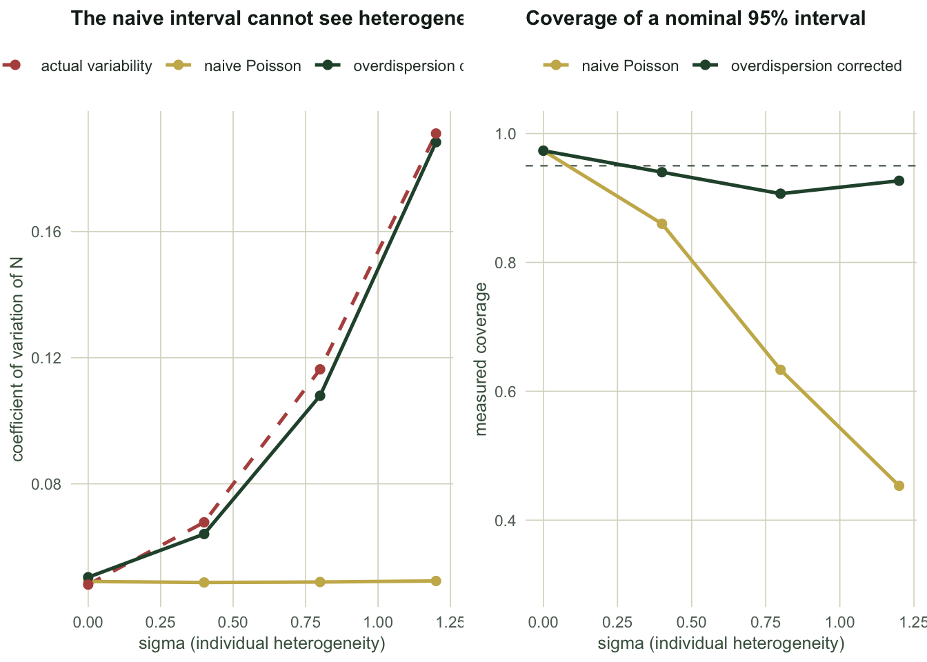
Read the `cv_naive` column downwards. It is `r sprintf("%.4f", sw$cv_naive[1])`, then `r sprintf("%.4f", sw$cv_naive[2])`, then `r sprintf("%.4f", sw$cv_naive[3])`, then `r sprintf("%.4f", sw$cv_naive[4])`. It holds to three decimals. Now read `cv_true` beside it: `r sprintf("%.4f", sw$cv_true[1])` rising to `r sprintf("%.4f", sw$cv_true[4])`, roughly a factor of `r sprintf("%.1f", sw$cv_true[4] / sw$cv_true[1])`.
The naive interval has no channel through which heterogeneity could reach it. It is computed from counts, and the counts look the same whether they came from four hundred identical animals or from four hundred wildly different ones. Coverage falls from `r sprintf("%.3f", sw$cover_naive[1])` to `r sprintf("%.3f", sw$cover_naive[4])` while the formula's reported precision holds to three decimals throughout. At the far end you are quoting a 95% interval that is really a `r sprintf("%.0f%%", 100 * sw$cover_naive[4])` interval.
The corrected version tracks: `cv_honest` climbs from `r sprintf("%.4f", sw$cv_honest[1])` to `r sprintf("%.4f", sw$cv_honest[4])`, following the truth, and coverage stays near nominal.
```{r fig-sweep}
#| echo: false
#| fig-width: 9.5
#| fig-cap: "Left: the naive coefficient of variation is flat across heterogeneity while the true one rises. Right: the resulting coverage of a nominal 95% interval."
#| fig-alt: "Two panels against sigma from zero to 1.2. Left panel: a flat gold line near 0.05 for the naive coefficient of variation, a rising green line for the honest one, and a rising dashed line for the true variability, with the gold line diverging further at each step. Right panel: coverage, the gold naive line falling from 0.97 to about 0.45 while the green honest line stays near the dashed nominal 0.95 as sigma rises rather than falling with the gold one."
library(ggplot2)
theme_te <- function() {
theme_minimal(base_size = 11) +
theme(
plot.background = element_rect(fill = "#f5f4ee", colour = NA),
panel.background = element_rect(fill = "#f5f4ee", colour = NA),
panel.grid.minor = element_blank(),
panel.grid.major = element_line(colour = "#dad9ca", linewidth = 0.3),
plot.title = element_text(colour = "#16241d", face = "bold", size = 11),
axis.title = element_text(colour = "#46604a", size = 9.5),
axis.text = element_text(colour = "#5d6b61", size = 8.5),
legend.position = "top", legend.title = element_blank(),
legend.text = element_text(colour = "#2c3a31", size = 8.5))
}
d1 <- rbind(
data.frame(s = sw$sigma, v = sw$cv_naive, k = "naive Poisson"),
data.frame(s = sw$sigma, v = sw$cv_honest, k = "overdispersion corrected"),
data.frame(s = sw$sigma, v = sw$cv_true, k = "actual variability"))
pA <- ggplot(d1, aes(s, v, colour = k, linetype = k)) +
geom_line(linewidth = 0.9) + geom_point(size = 2) +
scale_colour_manual(values = c("naive Poisson" = "#c9b458",
"overdispersion corrected" = "#275139",
"actual variability" = "#b5534e")) +
scale_linetype_manual(values = c("naive Poisson" = "solid",
"overdispersion corrected" = "solid",
"actual variability" = "dashed")) +
labs(title = "The naive interval misses heterogeneity",
x = "sigma (individual heterogeneity)", y = "coefficient of variation of N") +
theme_te()
d2 <- rbind(data.frame(s = sw$sigma, v = sw$cover_naive, k = "naive Poisson"),
data.frame(s = sw$sigma, v = sw$cover_honest, k = "overdispersion corrected"))
pB <- ggplot(d2, aes(s, v, colour = k)) +
geom_hline(yintercept = 0.95, linetype = "dashed", colour = "#5d6b61", linewidth = 0.4) +
geom_line(linewidth = 0.9) + geom_point(size = 2) +
scale_colour_manual(values = c("naive Poisson" = "#c9b458",
"overdispersion corrected" = "#275139")) +
scale_y_continuous(limits = c(0.3, 1)) +
labs(title = "Coverage of a nominal 95% interval",
x = "sigma (individual heterogeneity)", y = "measured coverage") +
theme_te()
grid::grid.newpage()
grid::pushViewport(grid::viewport(layout = grid::grid.layout(1, 2)))
print(pA, vp = grid::viewport(layout.pos.row = 1, layout.pos.col = 1))
print(pB, vp = grid::viewport(layout.pos.row = 1, layout.pos.col = 2))
```
## The honest limit
Everything above rests on one assumption that no diagnostic in the analysis can test: that the marked animals are a fair sample of the sighting process for the unmarked ones.
They are the only animals you can measure individually. Sigma comes from them; the overdispersion correction comes from them; the mean rate that divides the unmarked total comes from them. If collaring changes how visible an animal is, in either direction, all of it is measured on a population that does not exist outside the collars.
Here is what that costs. Suppose the collar makes an animal slightly less likely to be noticed, with a multiplier on its sighting rate.
```{r collar}
sim_eta <- function(N = 400, n = 80, J = 12, lam = 0.35, sigma = 0.8, eta = 1, seed = 1) {
  set.seed(seed)
  alpha <- rlnorm(N, log(lam) - sigma^2 / 2, sigma)
  mk <- sample(N, n)
  a2 <- alpha; a2[mk] <- a2[mk] * eta           # the collar effect, marked only
  y <- matrix(rpois(N * J, rep(a2, J)), N, J)
  list(N = N, n = n, J = J, ym = y[mk, , drop = FALSE], Tu = sum(y[-mk, , drop = FALSE]))
}
collar_row <- function(eta, R = 120) {
  r <- t(sapply(1:R, function(i) {
    dd <- sim_eta(eta = eta, seed = 7000 + i)
    out <- fit_one(dd)
    c(out, ratio = var(rowSums(dd$ym)) / mean(rowSums(dd$ym)))
  }))
  data.frame(eta = eta, mean_N = mean(r[, "N"]), bias = 100 * (mean(r[, "N"]) / 400 - 1),
             var_mean_ratio = mean(r[, "ratio"]), sigma_hat = mean(r[, "sigma"]))
}
cs <- do.call(rbind, lapply(c(1.0, 0.9, 0.8, 0.7), collar_row))
p314_cs <- cs
print(round(cs, 3), row.names = FALSE)
```
A ten per cent reduction in sightability produces a `r sprintf("%+.0f%%", cs$bias[2])` error in abundance. Thirty per cent produces `r sprintf("%+.0f%%", cs$bias[4])`. The direction is fixed: undercounting the marked animals makes the estimated rate too low, which makes the unmarked population look larger.
And now the part to remember. Look at `sigma_hat` down that table: `r sprintf("%.3f", cs$sigma_hat[1])`, `r sprintf("%.3f", cs$sigma_hat[2])`, `r sprintf("%.3f", cs$sigma_hat[3])`, `r sprintf("%.3f", cs$sigma_hat[4])`. It drifts downwards. What it is estimating does not: the collar effect is a constant multiplier on the marked animals' rates, and multiplying a log-normal by a constant moves its log-mean and leaves its log-sd, so the spread the likelihood targets is the same in all four rows. The overdispersion ratio sits above the Poisson value of 1 the whole way down. Neither `sigma_hat` nor the overdispersion ratio tells you the abundance is off by a third.
This is not a flaw in the estimator. It is the shape of the information: a rate measured on one group, applied to another, with nothing in the data connecting the two. The defence is design, not analysis. Collars that do not change behaviour, a marking period long enough for animals to settle, and a marked sample drawn the same way as the population you are counting.
## What to report
The abundance estimate, the sigma, the variance-to-mean ratio of the marked totals, and the interval computed with the overdispersion in it. If sigma is near zero the correction costs you nothing, as the sweep shows at the top row. If it is not, the correction is the difference between an interval and a decoration.
## Where to go next
If your animals are individually identifiable at every encounter, you want [closed capture-recapture](../closed-capture-recapture/), where the heterogeneity problem bites the estimate hard rather than the interval. If none of them are marked, [the random encounter model](../random-encounter-model-camera-traps/) gets density from sighting rates alone, at the cost of needing animal speed. If you can use the locations of the sightings as well as their counts, [spatial capture-recapture](../spatial-capture-recapture-basics/) uses far more of the information in the same field effort.
## References
McClintock, White, Antolin & Tripp 2009 Biometrics 65(1):237-246 (10.1111/j.1541-0420.2008.01047.x)
McClintock, White & Burnham 2006 Journal of Agricultural, Biological, and Environmental Statistics 11(3):231-248 (10.1198/108571106X129171)
McClintock & White 2009 Ecology 90(2):313-320 (10.1890/08-0973.1)
McClintock, White & Pryde 2019 Biometrics 75(3):799-809 (10.1111/biom.13058)
Bowden & Kufeld 1995 Journal of Wildlife Management 59(4):840-851 (10.2307/3801965)
Royle, Chandler, Sollmann & Gardner 2014 Spatial Capture-Recapture, ISBN 978-0-12-405939-9
## Related tutorials
- [Closed population capture-recapture in R](../closed-capture-recapture/)
- [The random encounter model for camera traps](../random-encounter-model-camera-traps/)
- [Spatial capture-recapture from scratch](../spatial-capture-recapture-basics/)
- [Capture heterogeneity: Mt, Mb and Mh in R](../capture-heterogeneity-mt-mb-mh/)