num <- integrate(function(a) pmax(0, -cos(a)) / (2 * pi), 0, 2 * pi)$value
c(numeric = num, closed_form = 1 / pi, gap = num - 1 / pi)
numeric closed_form gap
0.3183099 0.3183099 0.0000000 Corrected 14 October 2026: the take-away said the counting error is usually the least of the uncertainty in a random encounter model estimate, which the post never shows and its own path persistence sweep argues against; it now says the counting error comes on top of the auxiliary terms and is larger than a Poisson count would suggest when the animals wander.
Corrected 1 October 2026: the perimeter figure’s caption called its points means over the simulated animals, when they are encounter rates summed over all of them; and the closing note said the burst filter’s threshold has no correct value, where it now says the threshold should sit near the sensor’s own recovery time, as the checking post explains.
Corrected 27 September 2026: the post likened one deviation beyond two standard errors among five comparisons to a head among five coin flips, which made it sound almost certain; by chance alone it turns up far less often than that, though often enough that a single one is no surprise, and the sentence now says so.
A camera trap array gives you triggers. If the animals carry natural marks you can turn triggers into density with spatial capture-recapture. If they do not, the usual fallback is occupancy, which answers a different question, or a relative abundance index, which answers no question at all without a calibration you do not have.
The random encounter model (Rowcliffe et al. 2008) is the third option. It says that a camera is a small window onto a moving population, and that the rate at which animals walk through that window is a known function of how many there are, how fast they move, and how big the window is. Rearrange, and you get density from trigger counts.
The formula is short enough to fit in a sentence:
\[\frac{y}{t} = D \, v \, \frac{r(2 + \theta)}{\pi}\]
where \(y\) is the number of encounters over survey time \(t\), \(D\) is density, \(v\) is average speed, and \(r\) and \(\theta\) are the radius and angle of the detection zone. This post does three things with it: derives the constant, checks it against a simulation where the truth is known, and measures what the encounter rate alone can and cannot tell you.
Treat the animals as an ideal gas: density \(D\) per unit area, each moving at speed \(v\) in a direction that is uniformly distributed and independent of where it is. Hutchinson and Waser (2007) trace this idea through the encounter-rate literature, and it is the whole engine here.
Now put a fixed region in the middle of the gas and ask how often something walks into it. Take a short piece of the region’s boundary, length \(\mathrm{d}s\), with outward normal \(\mathbf{n}\). An animal crosses inwards through it at rate \(D \, \mathbb{E}[\max(0, -\mathbf{v} \cdot \mathbf{n})] \, \mathrm{d}s\): only the inward part of the velocity counts. With the direction uniform, that expectation is \(v\) times a pure number:
\[\mathbb{E}[\max(0, -\cos\psi)] = \frac{1}{2\pi}\int_0^{2\pi} \max(0, -\cos\psi) \, \mathrm{d}\psi = \frac{1}{\pi}\]
num <- integrate(function(a) pmax(0, -cos(a)) / (2 * pi), 0, 2 * pi)$value
c(numeric = num, closed_form = 1 / pi, gap = num - 1 / pi) numeric closed_form gap
0.3183099 0.3183099 0.0000000 So the inward flux is \(D v / \pi\) per unit of boundary, and the total entry rate is that times the boundary length:
\[\frac{y}{t} = \frac{D \, v \, L}{\pi}\]
That is the whole model. The famous \((2 + \theta)\) is not a fact about cameras; it is the perimeter of a circular sector of radius \(r\) and angle \(\theta\), which is two radii plus an arc:
\[L = 2r + r\theta = r(2 + \theta)\]
Two consequences fall straight out, and both are testable. A zone’s shape does not matter beyond its perimeter, so a wide shallow zone and a narrow deep one with the same perimeter give the same trigger rate. And a camera with a full 360 degree field of view has no radii at all, so its perimeter is \(2\pi r\) and its constant is \(2\pi\), not \(2 + 2\pi\).
To test the formula I need a simulation that counts crossings without approximating them. The trap is to sample the animal’s position on a time grid and count the steps where it flips from outside to inside: that silently misses every visit that starts and ends between two grid points, and the miss rate depends on the step length, which is the thing under test.
So the crossings get solved for. The detection zone points along the positive x axis and spans angles \(\pm\theta/2\). Its boundary has three pieces: an arc and two radii. For a straight step from P1 to P1 + D, each piece gives a quadratic or a linear equation, and each solution is an entry if the step points against the outward normal there.
## exact boundary crossings of the segments P1 -> P1 + D
## returns, per segment, up to 4 crossing positions u and whether each is inward
crossings <- function(P1, D, r, half) {
  m <- nrow(P1)
  U <- matrix(Inf, m, 4); IN <- matrix(FALSE, m, 4)

  ## the arc: |P1 + u D| = r, and the crossing point inside the angular span
  a <- D[, 1]^2 + D[, 2]^2
  b <- 2 * (P1[, 1] * D[, 1] + P1[, 2] * D[, 2])
  cc <- P1[, 1]^2 + P1[, 2]^2 - r^2
  disc <- b^2 - 4 * a * cc
  ok <- disc > 0 & a > 0
  sq <- ifelse(ok, sqrt(pmax(disc, 0)), NA_real_)
  for (k in 1:2) {
    u <- (-b + c(-1, 1)[k] * sq) / (2 * a)
    Q <- cbind(P1[, 1] + u * D[, 1], P1[, 2] + u * D[, 2])
    good <- ok & !is.na(u) & u > 0 & u <= 1 & abs(atan2(Q[, 2], Q[, 1])) <= half
    good[is.na(good)] <- FALSE
    U[good, k] <- u[good]                             # outward normal is Q / r
    IN[good, k] <- ((D[, 1] * Q[, 1] + D[, 2] * Q[, 2]) < 0)[good]
  }
  ## the two radii: the segments from the origin at +half and -half, out to r
  for (k in 1:2) {
    s <- c(1, -1)[k] * half
    e <- c(cos(s), sin(s))
    n <- c(cos(s + c(1, -1)[k] * pi / 2), sin(s + c(1, -1)[k] * pi / 2))
    cP <- P1[, 1] * e[2] - P1[, 2] * e[1]
    cD <- D[, 1] * e[2] - D[, 2] * e[1]
    u <- -cP / cD
    tt <- (P1[, 1] + u * D[, 1]) * e[1] + (P1[, 2] + u * D[, 2]) * e[2]
    good <- abs(cD) > 1e-12 & !is.na(u) & u > 0 & u <= 1 & tt >= 0 & tt <= r
    good[is.na(good)] <- FALSE
    U[good, 2 + k] <- u[good]
    IN[good, 2 + k] <- ((D[, 1] * n[1] + D[, 2] * n[2]) < 0)[good]
  }
  list(U = U, IN = IN)
}
The animals walk on a torus, so there are no edges to worry about and the stationary state is exactly the ideal gas: position uniform, direction uniform, the two independent. Turning angles come from a wrapped Cauchy with mean resultant length rho, which is a one-line inverse-CDF draw and gives everything from a uniform turn (rho = 0) to a nearly straight line (rho near 1).
walk_one <- function(nstep, dt, v, W, r, half, rho) {
  u <- runif(nstep)
  turn <- if (rho < 1e-9) 2 * pi * u - pi else
    2 * atan(((1 - rho) / (1 + rho)) * tan(pi * (u - 0.5)))
  phi <- runif(1, 0, 2 * pi) + cumsum(turn)
  D <- cbind(v * dt * cos(phi), v * dt * sin(phi))
  p0 <- c(runif(1, -W / 2, W / 2), runif(1, -W / 2, W / 2))
  X <- p0[1] + cumsum(D[, 1]); Y <- p0[2] + cumsum(D[, 2])
  P1 <- cbind(c(p0[1], X[-nstep]), c(p0[2], Y[-nstep]))
  R1 <- cbind(((P1[, 1] + W / 2) %% W) - W / 2, ((P1[, 2] + W / 2) %% W) - W / 2)
  idx <- which((R1[, 1]^2 + R1[, 2]^2) < (r + v * dt)^2)   # only steps near the zone
  if (!length(idx)) return(list(t_in = numeric(0), t_out = numeric(0)))
  cr <- crossings(R1[idx, , drop = FALSE], D[idx, , drop = FALSE], r, half)
  hit <- which(is.finite(cr$U), arr.ind = TRUE)
  if (!nrow(hit)) return(list(t_in = numeric(0), t_out = numeric(0)))
  tt <- (idx[hit[, 1]] - 1 + cr$U[hit]) * dt
  o <- order(tt); tt <- tt[o]; inw <- cr$IN[hit][o]
  list(t_in = tt[inw], t_out = tt[!inw])
}

## n independent animals on the same torus: that is the gas, at density n / W^2
gas <- function(n, nstep, dt, v, W, r, half, rho) {
  vapply(seq_len(n), function(i)
    length(walk_one(nstep, dt, v, W, r, half, rho)$t_in), numeric(1))
}Four detection angles, from a narrow 20 degree wedge to a 200 degree zone that is not even convex, plus a full circle for the limiting case. The prediction is \(D v L / \pi\) in every case, with \(L\) read off the geometry.
A word on the numbers before they appear. The simulated world is a 20 metre torus holding 120 animals, which is an absurd density for anything larger than a beetle. That is deliberate, and it costs nothing: the formula has no scale in it, so multiplying \(D\) by a thousand multiplies \(y\) by a thousand and leaves every ratio below untouched. A ridiculous density buys encounters in seconds instead of decades. Field units come back at the end.
W <- 20; r <- 4; v <- 1; dt <- 0.5; nanim <- 120; nstep <- 25000
A <- W^2; Tt <- nstep * dt; Dtrue <- nanim / A

set.seed(3001)
thd <- c(20, 60, 120, 200)
res <- do.call(rbind, lapply(thd, function(th) {
  half <- (th / 2) * pi / 180
  y <- gas(nanim, nstep, dt, v, W, r, half, rho = 0.9)
  L <- 2 * r + 2 * r * half
  data.frame(zone = paste0(th, " deg"), L = L,
             obs = sum(y) / Tt, se = sd(y / Tt) * sqrt(nanim),
             pred = Dtrue * v * L / pi)
}))
res$ratio <- res$obs / res$pred
res
zone L obs se pred ratio
1 20 deg 9.396263 0.90112 0.009936901 0.8972771 1.0042829
2 60 deg 12.188790 1.16976 0.010231120 1.1639437 1.0049970
3 120 deg 16.377580 1.53856 0.011129710 1.5639437 0.9837694
4 200 deg 21.962634 2.08976 0.011589473 2.0972771 0.9964158## a full circle has no radii, so its perimeter is 2 pi r and its constant is 2 pi
walk_disc <- function(nstep, dt, v, W, r, rho) {
u <- runif(nstep)
turn <- 2 * atan(((1 - rho) / (1 + rho)) * tan(pi * (u - 0.5)))
phi <- runif(1, 0, 2 * pi) + cumsum(turn)
D <- cbind(v * dt * cos(phi), v * dt * sin(phi))
p0 <- c(runif(1, -W / 2, W / 2), runif(1, -W / 2, W / 2))
X <- p0[1] + cumsum(D[, 1]); Y <- p0[2] + cumsum(D[, 2])
P1 <- cbind(c(p0[1], X[-nstep]), c(p0[2], Y[-nstep]))
R1 <- cbind(((P1[, 1] + W / 2) %% W) - W / 2, ((P1[, 2] + W / 2) %% W) - W / 2)
a <- D[, 1]^2 + D[, 2]^2
b <- 2 * (R1[, 1] * D[, 1] + R1[, 2] * D[, 2])
cc <- R1[, 1]^2 + R1[, 2]^2 - r^2
disc <- b^2 - 4 * a * cc
n <- 0
for (k in 1:2) {
uu <- (-b + c(-1, 1)[k] * sqrt(pmax(disc, 0))) / (2 * a)
Q <- cbind(R1[, 1] + uu * D[, 1], R1[, 2] + uu * D[, 2])
n <- n + sum(disc > 0 & uu > 0 & uu <= 1 &
(D[, 1] * Q[, 1] + D[, 2] * Q[, 2]) < 0, na.rm = TRUE)
}
n
}
set.seed(3002)
ydisc <- vapply(seq_len(nanim), function(i) walk_disc(nstep, dt, v, W, r, 0.9), numeric(1))
disc <- data.frame(zone = "360 deg", L = 2 * pi * r, obs = sum(ydisc) / Tt,
se = sd(ydisc / Tt) * sqrt(nanim),
pred = Dtrue * v * (2 * pi * r) / pi)
disc$ratio <- disc$obs / disc$pred
disc zone L obs se pred ratio
1 360 deg 25.13274 2.39928 0.01221001 2.4 0.9997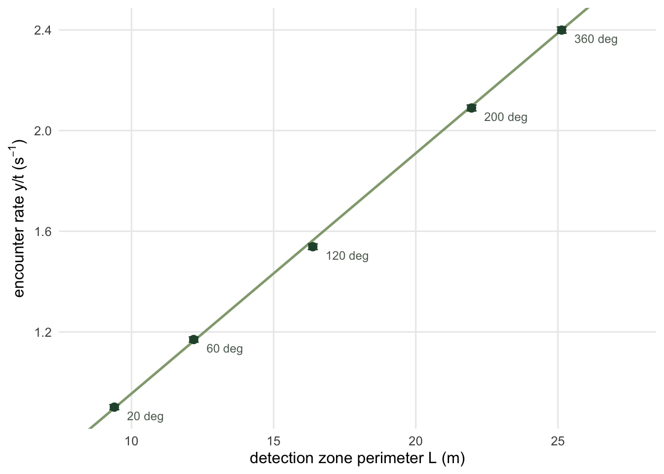
observed / predicted, five zones: 0.9838 to 1.0050deviations in standard errors: +0.39, +0.57, -2.28, -0.65, -0.06pooled against the theory: sum of squared z = 6.10 on 5 df, p = 0.297The ratio of observed to predicted rate stays between 0.984 and 1.005 across detection angles from 20 to 360 degrees, a perimeter range of 9.4 to 25.1 metres, and pooled across the five zones the deviations are what Monte Carlo error alone produces (p = 0.30). Read the individual standard errors with that in mind: five comparisons will fairly often throw up one deviation beyond two standard errors by chance alone, so a single one is no surprise. The 200 degree zone is worth a second look: it is not convex, an animal can leave through one radius and come straight back in through the other, and the perimeter rule holds anyway. The flux argument never needed convexity, because it is local to each piece of boundary.
The derivation asked for one thing about the movement: that the direction is uniform and independent of position. It said nothing about persistence. A nearly straight-line traveller and a drunkard that reverses at every step should trigger the camera at the same rate, as long as their speed along the path is the same.
That is not intuitive. A wandering animal spends longer in the neighbourhood of the camera, so it feels like it should be recorded more. Here is the measurement.
half40 <- 20 * pi / 180
L40 <- 2 * r + 2 * r * half40
pred40 <- Dtrue * v * L40 / pi
set.seed(3003)
rhos <- c(0, 0.5, 0.9, 0.98)
tor <- do.call(rbind, lapply(rhos, function(rh) {
  y <- gas(nanim, nstep, dt, v, W, r, half40, rho = rh)
  data.frame(rho = rh, obs = sum(y) / Tt, se = sd(y / Tt) * sqrt(nanim))
}))
tor$ratio <- tor$obs / pred40
tor$rel_se <- tor$se / pred40
tor
rho obs se ratio rel_se
1 0.00 1.00008 0.028816726 0.9703764 0.027960834
2 0.50 1.04424 0.018680523 1.0132248 0.018125688
3 0.90 1.04984 0.009488288 1.0186585 0.009206475
4 0.98 1.03032 0.008096092 0.9997182 0.007855628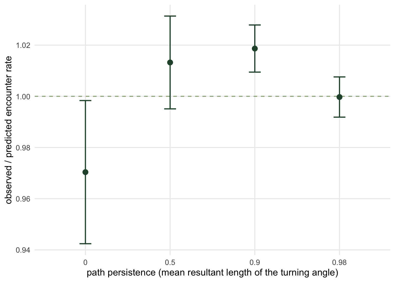
deviations in standard errors: -1.06, +0.73, +2.03, -0.04pooled: sum of squared z = 5.76 on 4 df, p = 0.218standard error, rho = 0 relative to rho = 0.98: 3.56 timesAll four sit on the theory (pooled p = 0.22). What changes is the precision: the standard error is 3.6 times larger for the uniform-turn walker than for the nearly straight one, on identical survey effort. The mean is right and the variance is not what a Poisson count would give you, because a tortuous animal crosses the boundary several times per visit and those crossings are anything but independent. Treat that as a warning about confidence intervals rather than about the point estimate.
Rearranged, the model is a single ratio.
th40 <- 2 * half40
yy <- sum(gas(nanim, nstep, dt, v, W, r, half40, rho = 0.9))
rem_D <- function(y, t, v, r, theta) y * pi / (t * v * r * (2 + theta))
Dhat <- rem_D(yy, Tt, v, r, th40)
c(y = yy, D_hat = Dhat, D_true = Dtrue, ratio = Dhat / Dtrue)
y D_hat D_true ratio
1.297700e+04 3.021976e-01 3.000000e-01 1.007325e+00 With the truth handed to it, the estimator returns 0.3022 animals per square metre against a true 0.3000. That is the easy part. The hard part is what happens when the speed is wrong.
  v_assumed     D_hat ratio_to_truth
1      0.50 0.6043952      2.0146507
2      0.80 0.3777470      1.2591567
3      1.00 0.3021976      1.0073254
4      1.25 0.2417581      0.8058603
5      2.00 0.1510988      0.5036627
The encounter rate is a function of the product \(Dv\), and nothing else. Halve the assumed speed and the density doubles, exactly; there is no partial cancellation and no diagnostic on the trigger counts that will tell you which factor moved. This is not a weakness of the fit, it is the identity that makes the method work: the camera measures a flux, and a flux is a density times a velocity. The whole method therefore rests on getting \(v\) from somewhere else, and \(r\) and \(\theta\) from somewhere else, and the honest accounting is that a camera trap survey using the random encounter model is three surveys wearing one coat.
Which is not a reason to avoid it. Spatial capture-recapture also rests on assumptions you cannot check from the detections alone; the difference is that the random encounter model wears its external inputs on the outside of the formula where you can argue about them.
The torus was a test rig. The same three lines run on a real survey: 60 cameras out for 30 days, 200 encounters in total, a detection zone measured at 10 metres by 40 degrees, and a day range of 3.5 km taken from telemetry on the same population.
y_field <- 200
t_field <- 60 * 30                      # camera-days
v_field <- 3.5                          # km per day
r_field <- 0.010                        # km
th_field <- 40 * pi / 180               # radians
D_field <- rem_D(y_field, t_field, v_field, r_field, th_field)
c(D_per_km2 = D_field, animals_in_100km2 = D_field * 100)
D_per_km2 animals_in_100km2
3.696376 369.637628 That is 3.70 animals per square kilometre. Now perturb the inputs the way a real survey perturbs them: the day range is uncertain by a factor of 1.3 either way, and the detection radius by 2 metres.
         v     r        D     ratio
9 4.550000 0.012 2.369472 0.6410256
6 4.550000 0.010 2.843366 0.7692308
8 3.500000 0.012 3.080314 0.8333333
3 4.550000 0.008 3.554208 0.9615385
5 3.500000 0.010 3.696376 1.0000000
7 2.692308 0.012 4.004408 1.0833333
2 3.500000 0.008 4.620470 1.2500000
4 2.692308 0.010 4.805289 1.3000000
1 2.692308 0.008 6.006611 1.6250000
The density spans a factor of 2.5 across that box, and every cell of it is an equally defensible answer given the equally defensible inputs. No amount of extra camera-nights narrows it, because the width comes from \(v\) and \(r\), not from \(y\). If you take one thing from this post, take that: the interval on a random encounter model estimate is in large part an interval on the auxiliary measurements, and the counting error comes on top of that, larger than a Poisson count would suggest when the animals wander, as the path persistence sweep showed. The checking post builds the interval properly.
The speed is the input people get wrong, and the way they get it wrong is systematic rather than sloppy: camera-derived speeds are sampled with probability proportional to speed, so the obvious average is biased upwards by a factor you can write down. That is the next post. After that, the staying time offers a way to sidestep the speed measurement entirely, using the same geometry read in the other direction.
One practical note before you fit this to real data: the derivation counts boundary crossings, and a camera delivers photo bursts. Turning bursts into encounters means a filter, and its threshold should be set to something like the sensor’s own recovery time. The checking post measures what a wrong threshold costs.
Newsletter
Get updates by email
An occasional email when tutorials are added or substantially corrected. No spam; unsubscribe anytime.
By subscribing you agree to receive these emails and confirm your address once. See the privacy policy.