inside <- function(P, r, half) {
  (P[, 1]^2 + P[, 2]^2 <= r^2) & (abs(atan2(P[, 2], P[, 1])) <= half)
}

crossings <- function(P1, D, r, half) {
  m <- nrow(P1)
  U <- matrix(Inf, m, 4); IN <- matrix(FALSE, m, 4)
  a <- D[, 1]^2 + D[, 2]^2
  b <- 2 * (P1[, 1] * D[, 1] + P1[, 2] * D[, 2])
  cc <- P1[, 1]^2 + P1[, 2]^2 - r^2
  disc <- b^2 - 4 * a * cc
  ok <- disc > 0 & a > 0
  sq <- ifelse(ok, sqrt(pmax(disc, 0)), NA_real_)
  for (k in 1:2) {                                        # the arc
    u <- (-b + c(-1, 1)[k] * sq) / (2 * a)
    Q <- cbind(P1[, 1] + u * D[, 1], P1[, 2] + u * D[, 2])
    good <- ok & !is.na(u) & u > 0 & u <= 1 & abs(atan2(Q[, 2], Q[, 1])) <= half
    good[is.na(good)] <- FALSE
    U[good, k] <- u[good]
    IN[good, k] <- ((D[, 1] * Q[, 1] + D[, 2] * Q[, 2]) < 0)[good]
  }
  for (k in 1:2) {                                        # the two radii
    s <- c(1, -1)[k] * half
    e <- c(cos(s), sin(s))
    nrm <- c(cos(s + c(1, -1)[k] * pi / 2), sin(s + c(1, -1)[k] * pi / 2))
    cD <- D[, 1] * e[2] - D[, 2] * e[1]
    u <- -(P1[, 1] * e[2] - P1[, 2] * e[1]) / cD
    tt <- (P1[, 1] + u * D[, 1]) * e[1] + (P1[, 2] + u * D[, 2]) * e[2]
    good <- abs(cD) > 1e-12 & !is.na(u) & u > 0 & u <= 1 & tt >= 0 & tt <= r
    good[is.na(good)] <- FALSE
    U[good, 2 + k] <- u[good]
    IN[good, 2 + k] <- ((D[, 1] * nrm[1] + D[, 2] * nrm[2]) < 0)[good]
  }
  list(U = U, IN = IN)
}Staying time and the REST model in R
R
camera traps
abundance
movement ecology
ecology tutorial
The REST model estimates animal density from how long animals stay in view, with no external speed. Little’s law and Cauchy’s chord identity, tested in R.
Corrected 25 September 2026: this post said that extrapolating the clipped tail with a parametric survival model is what a serious analysis does. Measured on the post’s own data, the family AIC prefers stays near half the true density at every clip length and falls behind the plain truncated mean from 60 seconds; only a two-part mixture recovers it. The section “The camera has a stopwatch with a limit” now shows both.
The random encounter model has one weak joint: it needs the average speed, and the average has to include every hour the animal spends lying still. You cannot get that from the camera without an assumption about activity, and you cannot get it from a GPS collar without collaring something.
The random encounter and staying time model (Nakashima et al. 2018) removes that joint. It uses the same cameras and the same triggers, but instead of asking how fast animals cross the detection zone it asks how long they stay in it. The estimator is:
\[D = \frac{y}{t} \cdot \frac{\mathbb{E}[T_{\text{stay}}]}{a}\]
where \(a\) is the area of the detection zone and \(T_{\text{stay}}\) is the time an animal spends in view per visit. No speed. No activity level. Both are measured for you, implicitly, by the stopwatch.
Why that works: Little’s law
The formula is not a camera trap result at all. It is Little’s law, which says that for any stable system, the average number of customers inside equals the arrival rate times the average time each one spends there. Queueing theorists have used it since 1961 to reason about supermarket tills.
Point it at a detection zone. The average number of animals inside is \(D a\), because the gas is uniform. The arrival rate is \(y/t\). The average time each one spends there is \(\mathbb{E}[T_{\text{stay}}]\). So
\[D a = \frac{y}{t}\,\mathbb{E}[T_{\text{stay}}]\]
and that is the whole derivation. Notice what is not in it: no assumption about how the animals move, no speed, no direction distribution, not even the shape of the zone. Little’s law needs stationarity and nothing else.
Set it beside the random encounter model (Rowcliffe et al. 2008; the ideal gas model behind it is reviewed by Hutchinson and Waser 2007), which says \(y/t = D v r(2+\theta)/\pi\), and one substitution gives a prediction about staying time:
\[\mathbb{E}[T_{\text{stay}}] = \frac{\pi a}{v L}, \qquad L = r(2+\theta)\]
That is Cauchy’s mean chord formula wearing a wildlife hat: the average chord an isotropic straight line cuts across a convex region has length \(\pi a / L\), and dividing by speed turns a length into a time. So the two models are the same equation read in two directions. The random encounter model measures \(v\) elsewhere and predicts the count; the staying time model measures the count and the clock, and lets them tell it about \(v\).
The rig
Same gas as the encounter rate post: independent walkers on a torus, exact boundary crossings, no time-step discretisation to apologise for. The extra piece here is the stopwatch.
An animal is active or resting, switching between the two as a Markov chain on the step grid. Resting means the step length is zero, which the crossing routine handles for free: a zero-length segment cannot cross anything. The proportion of time active follows from the two switching probabilities.
walk_one <- function(nstep, dt, v, W, r, half, rho, p_ar = 0, p_ra = 1) {
  ## active / resting state sequence, built bout by bout (p_ar = 0 means never rests)
  st <- if (p_ar <= 0) rep(1L, nstep) else {
    z <- integer(0); s <- 1L
    while (length(z) < nstep) {
      z <- c(z, rep(s, rgeom(1, if (s == 1L) p_ar else p_ra) + 1L)); s <- 1L - s
    }
    z[seq_len(nstep)]
  }

  u <- runif(nstep)
  turn <- 2 * atan(((1 - rho) / (1 + rho)) * tan(pi * (u - 0.5)))
  phi <- runif(1, 0, 2 * pi) + cumsum(turn)
  step <- v * dt * st                                     # zero while resting
  D <- cbind(step * cos(phi), step * sin(phi))
  p0 <- c(runif(1, -W / 2, W / 2), runif(1, -W / 2, W / 2))
  X <- p0[1] + cumsum(D[, 1]); Y <- p0[2] + cumsum(D[, 2])
  P1 <- cbind(c(p0[1], X[-nstep]), c(p0[2], Y[-nstep]))
  R1 <- cbind(((P1[, 1] + W / 2) %% W) - W / 2, ((P1[, 2] + W / 2) %% W) - W / 2)

  frac_in <- mean(inside(R1, r, half))                    # time-average occupancy
  idx <- which((R1[, 1]^2 + R1[, 2]^2) < (r + v * dt)^2)
  if (!length(idx)) return(list(visits = numeric(0), frac_in = frac_in, active = mean(st)))
  cr <- crossings(R1[idx, , drop = FALSE], D[idx, , drop = FALSE], r, half)
  hit <- which(is.finite(cr$U), arr.ind = TRUE)
  if (!nrow(hit)) return(list(visits = numeric(0), frac_in = frac_in, active = mean(st)))
  tt <- (idx[hit[, 1]] - 1 + cr$U[hit]) * dt
  o <- order(tt); tt <- tt[o]; inw <- cr$IN[hit][o]
  t_in <- tt[inw]; t_out <- tt[!inw]
  if (!length(t_in)) return(list(visits = numeric(0), frac_in = frac_in, active = mean(st)))
  j <- findInterval(t_in, t_out) + 1L                     # the exit that closes each entry
  ok <- j <= length(t_out)                                # drop a visit still open at the end
  list(visits = t_out[j[ok]] - t_in[ok], frac_in = frac_in, active = mean(st))
}

gas <- function(n, nstep, dt, v, W, r, half, rho, p_ar = 0, p_ra = 1) {
  out <- lapply(seq_len(n), function(i) walk_one(nstep, dt, v, W, r, half, rho, p_ar, p_ra))
  list(visits = unlist(lapply(out, `[[`, "visits")),
       dur = vapply(out, function(z) sum(z$visits), numeric(1)),    # per animal
       nvis = vapply(out, function(z) length(z$visits), numeric(1)),
       frac_in = vapply(out, `[[`, numeric(1), "frac_in"),
       active = vapply(out, `[[`, numeric(1), "active"))
}

## the mean staying time is a ratio of two per-animal totals, so its standard error
## comes from resampling animals, which also allows for any clustering of visits
boot_stay <- function(g, B = 600) {
  n <- length(g$dur)
  vapply(seq_len(B), function(b) {
    i <- sample.int(n, n, replace = TRUE)
    sum(g$dur[i]) / sum(g$nvis[i])
  }, numeric(1))
}
Four identities, one simulation
Start with a gas that never rests. There are four claims stacked on top of each other and the simulation checks each one separately: that the gas really is uniform, that Little’s law holds, that the mean staying time matches Cauchy’s chord formula, and that the resulting density estimate is right.
W <- 20; r <- 4; half <- 20 * pi / 180; v <- 1; dt <- 0.5
A <- W^2; a_zone <- half * r^2; L <- 2 * r + 2 * r * half
nanim <- 120; nstep <- 20000; Tt <- nstep * dt; Dtrue <- nanim / A

set.seed(2701)
g <- gas(nanim, nstep, dt, v, W, r, half, rho = 0.9)
lambda <- length(g$visits) / Tt                    # arrivals per second, whole population
Wbar <- mean(g$visits)                             # mean staying time
Lnum <- sum(g$frac_in)                             # mean number inside, from positions

data.frame(
  claim = c("gas is uniform: mean number inside = D a",
            "Little's law: arrival rate x staying time = mean number inside",
            "Cauchy chord: mean staying time = pi a / (v L)",
            "REST estimate of density"),
  measured = c(Lnum, lambda * Wbar, Wbar, lambda * Wbar / a_zone),
  predicted = c(Dtrue * a_zone, Lnum, pi * a_zone / (v * L), Dtrue))
claim measured
1 gas is uniform: mean number inside = D a 1.6662000
2 Little's law: arrival rate x staying time = mean number inside 1.6673568
3 Cauchy chord: mean staying time = pi a / (v L) 1.6258964
4 REST estimate of density 0.2985391
predicted
1 1.675516
2 1.666200
3 1.625751
4 0.300000Every row lands. The third is the one worth pausing on: the mean staying time is 1.626 seconds against a predicted 1.626, and that prediction came from a nineteenth-century integral geometry result about random lines crossing a convex set.
Now vary the tortuosity. The encounter rate post showed that path persistence does not change how often animals arrive. Little’s law then forces something less obvious: it cannot change how long they stay either, because the occupancy and the arrival rate are both fixed, and the staying time is their ratio.
set.seed(2702)
tor <- do.call(rbind, lapply(c(0, 0.5, 0.9, 0.98), function(rh) {
  gg <- gas(150, nstep, dt, v, W, r, half, rho = rh)
  bs <- boot_stay(gg)
  data.frame(rho = rh, n_visits = length(gg$visits), mean_stay = mean(gg$visits),
             boot_se = sd(bs), CV_stay = sd(gg$visits) / mean(gg$visits))
}))
tor$predicted <- pi * a_zone / (v * L)
tor$ratio <- tor$mean_stay / tor$predicted
tor$z <- (tor$mean_stay - tor$predicted) / tor$boot_se
tor
rho n_visits mean_stay boot_se CV_stay predicted ratio z
1 0.00 13057 1.605594 0.019604282 1.2827629 1.625751 0.9876013 -1.02820780
2 0.50 12571 1.625056 0.012361039 0.8740768 1.625751 0.9995725 -0.05622141
3 0.90 12730 1.621472 0.008907677 0.6246751 1.625751 0.9973680 -0.48037764
4 0.98 12836 1.628164 0.008420554 0.5810123 1.625751 1.0014844 0.28658810The means agree to within 1.2 per cent across a walker that redraws its heading uniformly at every step and one that travels almost in a straight line, and the farthest sits 1.0 standard errors from the chord formula. The standard error comes from resampling animals, which is the safe default for a ratio of totals and which also allows for visits clustering within individuals. The coefficient of variation does not agree: it runs from 0.58 to 1.28. A tortuous animal delivers the same average visit through a wilder mixture of quick clips and long meanders, and that is variance you pay for in the interval, not in the estimate.
Where it earns its keep: resting animals
Now switch resting on. The animals are active 30 per cent of the time, in bouts of about a minute, with rests of about two minutes. Nothing else changes.
p_ra <- dt / 120                                  # mean rest bout 120 s
A_level <- 0.30
p_ar <- p_ra * (1 - A_level) / A_level            # gives 30 per cent active in the long run

set.seed(2703)
gr <- gas(nanim, nstep, dt, v, W, r, half, rho = 0.9, p_ar = p_ar, p_ra = p_ra)
lam_r <- length(gr$visits) / Tt
W_r <- mean(gr$visits)

rem_D <- function(y, t, vv, r, theta) y * pi / (t * vv * r * (2 + theta))
res <- data.frame(
  method = c("REST: (y/t) E[T] / a",
             "REM with the camera's active speed",
             "REM with the true time-averaged speed"),
  D_hat = c(lam_r * W_r / a_zone,
            rem_D(length(gr$visits), Tt, v, r, 2 * half),
            rem_D(length(gr$visits), Tt, v * mean(gr$active), r, 2 * half)))
res$ratio_to_truth <- res$D_hat / Dtrue
bs_r <- boot_stay(gr)
naive_se <- sd(gr$visits) / sqrt(length(gr$visits))    # pretends visits are independent
c(n_visits = length(gr$visits), realised_activity = mean(gr$active), mean_stay = W_r,
  boot_se = sd(bs_r), naive_se = naive_se, se_ratio = sd(bs_r) / naive_se,
  CV_stay = sd(gr$visits) / W_r, max_stay = max(gr$visits))
n_visits realised_activity mean_stay boot_se
3114.0000000 0.3028683 5.2183915 0.5915992
naive_se se_ratio CV_stay max_stay
0.5537578 1.0683357 5.9216465 695.7260233 res method D_hat ratio_to_truth
1 REST: (y/t) E[T] / a 0.29095640 0.9698547
2 REM with the camera's active speed 0.09064531 0.3021510
3 REM with the true time-averaged speed 0.29928950 0.9976317This is the argument for the staying time model in one table. The animals now spend 70 per cent of their lives motionless, and the staying time model does not care: it returns 0.97 times the truth, with a bootstrap standard error of 0.11 on the ratio, without being told the activity level, because a resting animal in the zone is still an animal in the zone and Little’s law counts it. Feed the random encounter model the speed the camera actually measures, which is the speed of moving animals, and it returns 0.30 times the truth. It only recovers once you hand it the activity level from somewhere else.
The bill arrives in the shape of the distribution. The coefficient of variation of the staying time has gone from about 0.6 to 5.9, and the longest single visit was 696 seconds against a mean of 5.2. The mean of that distribution is a rare-event statistic: most visits are quick transits, and the average is set by the handful that turned into a nap. Even with 3114 visits recorded, the standard error on the mean is 11 per cent, and it carries straight through to the density.
One thing is not driving that: clustering. Resampling animals rather than visits changes the standard error by a factor of 1.07, so the visits are close to independent here and the imprecision is the tail itself, not the clustering. Between-camera heterogeneity is a different matter, and the checking post deals with it.
The camera has a stopwatch with a limit
Which brings the whole thing down. A camera records a clip of fixed length, or a burst with a maximum, and any stay that outlasts it is cut off. Cut a distribution whose mean lives in its tail and you cut the mean.
caps <- c(5, 10, 30, 60, 120, Inf)
cens <- data.frame(setting = ifelse(is.finite(caps), paste0(caps, " s"), "no limit"),
                   cap = caps)
cens$mean_recorded <- vapply(caps, function(cap) mean(pmin(gr$visits, cap)), numeric(1))
cens$D_hat <- lam_r * cens$mean_recorded / a_zone
cens$ratio_to_truth <- cens$D_hat / Dtrue
cens$pct_visits_cut <- vapply(caps, function(cap) 100 * mean(gr$visits > cap), numeric(1))
cens[, c("setting", "mean_recorded", "D_hat", "ratio_to_truth", "pct_visits_cut")]
setting mean_recorded D_hat ratio_to_truth pct_visits_cut
1 5 s 1.713229 0.09552274 0.3184091 3.050739
2 10 s 1.851698 0.10324320 0.3441440 2.697495
3 30 s 2.356079 0.13136543 0.4378848 2.312139
4 60 s 2.970055 0.16559824 0.5519941 1.830443
5 120 s 3.843034 0.21427203 0.7142401 1.027617
6 no limit 5.218391 0.29095640 0.9698547 0.000000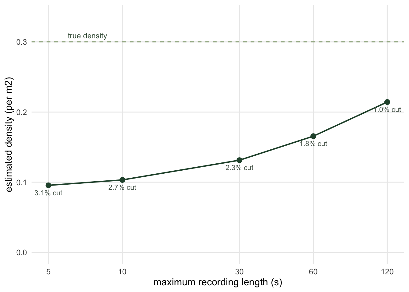
A 30 second clip recovers 44 per cent of the population while cutting only 2.3 per cent of the visits. That is the shape of the problem: the visits you lose are exactly the ones carrying the mean.
The instinct at this point is to reach for survival analysis, since these are textbook right-censored durations. Nonparametric survival analysis does not help, and the reason is worth understanding. When every observation is censored at the same known time \(c\), the Kaplan-Meier curve is just the empirical survival function up to \(c\) and stops. The restricted mean it gives you is \(\mathbb{E}[\min(T, c)]\), which is exactly the truncated mean in the table above. The tail beyond \(c\) is not poorly estimated, it is not estimated: nothing in the data speaks to it. You can bound \(D\) from below, and that is all.
Going past that bound takes an assumption about the tail. The usual one is a parametric survival model: fit several families to the censored stays with survreg and keep the one AIC prefers. The chunk below does that on the same draw at four clip lengths, and adds a censored two-part mixture of a lognormal and an exponential, fitted by maximum likelihood from six starting points that try both parts in both roles, since either can take the transits. It then resamples animals, as the bootstrap above did, and refits the mixture to each resample.
library(survival)
fams <- c("exponential", "weibull", "lognormal", "loglogistic")
fam_mean <- function(fit, dist) {                  # mean of the fitted distribution
  m <- unname(coef(fit)); s <- fit$scale
  switch(dist, exponential = exp(m), weibull = exp(m) * gamma(1 + s),
         lognormal = exp(m + s^2 / 2),
         loglogistic = if (s < 1) exp(m) * pi * s / sin(pi * s) else Inf)
}
mix_nll <- function(p, yo, yc) {                   # lognormal + exponential; yo seen to the end, yc cut
  w <- plogis(p[1]); s <- exp(p[3]); rt <- exp(p[4])
  dens <- (1 - w) * dlnorm(yo, p[2], s) + w * dexp(yo, rt)
  surv <- (1 - w) * plnorm(yc, p[2], s, lower.tail = FALSE) + w * pexp(yc, rt, lower.tail = FALSE)
  v <- -sum(log(pmax(dens, 1e-300))) - sum(log(pmax(surv, 1e-300)))
  if (is.finite(v)) v else 1e10
}
mix_fit <- function(y, d, which_starts = 1:6) {   # either part in either role, then a polish
  yo <- y[d == 1]; yc <- y[d == 0]; my <- log(median(y))
  starts <- list(c(-3, my, 0, log(1 / 30)), c(-2, my, -0.5, log(1 / 100)),    # 1-3: exponential long
                 c(-4, my, 0.3, log(1 / 300)), c(3, log(max(y)), 0, -my),      # 4-5: exponential short
                 c(3.5, log(max(y)) - 1, -0.5, -my), c(0.5, my, -1, -my))     # 6: both short
  fits <- lapply(starts[which_starts], function(st)
    optim(st, mix_nll, yo = yo, yc = yc, control = list(maxit = 2000)))
  p <- fits[[which.min(vapply(fits, `[[`, numeric(1), "value"))]]$par
  p <- optim(p, mix_nll, yo = yo, yc = yc, method = "BFGS")$par
  w <- plogis(p[1]); m_ln <- exp(p[2] + exp(p[3])^2 / 2); m_ex <- exp(-p[4])
  c(mean = (1 - w) * m_ln + w * m_ex, long_share = if (m_ex > m_ln) w else 1 - w,
    long_mean = max(m_ln, m_ex), nll = mix_nll(p, yo, yc))
}
to_truth <- function(m) lam_r * m / a_zone / Dtrue  # a mean stay as a ratio of density to truth

fit_caps <- c(10, 30, 60, 120)
fit_tab <- do.call(rbind, lapply(fit_caps, function(cap) {
  y <- pmin(gr$visits, cap); d <- as.integer(gr$visits < cap)
  fits <- lapply(fams, function(f) survreg(Surv(y, d) ~ 1, dist = f))
  best <- which.min(vapply(fits, AIC, numeric(1)))
  mx <- mix_fit(y, d)
  data.frame(setting = paste0(cap, " s"), truncated = to_truth(mean(y)), aic_family = fams[best],
             aic_best = to_truth(fam_mean(fits[[best]], fams[best])), mixture = to_truth(mx[["mean"]]),
             long_share = mx[["long_share"]], long_mean = mx[["long_mean"]], nll = mx[["nll"]])
}))
aic_same <- all(fit_tab$aic_family == fit_tab$aic_family[1])
fit_tab
setting truncated aic_family aic_best mixture long_share long_mean
1 10 s 0.3441440 loglogistic 0.4528642 0.3531475 0.31284298 2.181464
2 30 s 0.4378848 loglogistic 0.4739914 0.6176253 0.02623663 66.010283
3 60 s 0.5519941 loglogistic 0.4838850 0.9547062 0.02630168 134.841291
4 120 s 0.7142401 loglogistic 0.4889645 0.9779804 0.02630027 139.604512
nll
1 4730.231
2 4954.731
3 5043.808
4 5186.053## the 30 s fit again, started only with the exponential on the long stays
low30 <- mix_fit(pmin(gr$visits, 30), as.integer(gr$visits < 30), which_starts = 1:3)
c(low_peak_ratio = to_truth(low30[["mean"]]), nll_above_best = low30[["nll"]] - fit_tab$nll[2])low_peak_ratio nll_above_best
0.9354127 235.8884906 ## the spread: resample animals, refit the mixture, compare with the uncapped mean
by_animal <- split(gr$visits, factor(rep(seq_len(nanim), gr$nvis), levels = seq_len(nanim)))
n_refit <- 50
set.seed(2704)
refit <- t(vapply(seq_len(n_refit), function(b) {
xb <- unlist(by_animal[sample.int(nanim, nanim, replace = TRUE)], use.names = FALSE)
c(no_limit = mean(xb),
vapply(fit_caps[-1], function(cap) mix_fit(pmin(xb, cap), as.integer(xb < cap))[["mean"]], numeric(1)))
}, numeric(length(fit_caps))))
colnames(refit) <- c("no limit", paste0(fit_caps[-1], " s"))
refit_q <- apply(refit / W_r, 2, quantile, c(0.1, 0.5, 0.9, 1))
refit_q no limit 30 s 60 s 120 s
10% 0.8370421 0.5625549 0.7817688 0.8530294
50% 0.9818542 0.6424347 1.0004070 0.9737500
90% 1.1462935 0.8373653 1.3371902 1.1891348
100% 1.2351786 1.3183757 1.6379356 1.3776624The family AIC prefers is the loglogistic at every clip length, and its density hardly moves with the clip: 0.45 of the truth at 10 seconds and 0.49 at 120. Over the same range the plain truncated mean climbs from 0.34 to 0.71, so the fitted model is ahead of doing nothing at 10 and 30 seconds and behind it at 60 and 120. A single family spends its likelihood on the transits, which are nearly all of the visits, and extrapolates their tail. At 60 and 120 seconds its whole mean, tail included, is below the mean the camera actually recorded, so it does not even reproduce the long stays that were seen.
The two-part mixture recovers the density from 60 seconds up: 0.95 and 0.98 of the truth at 60 and 120 seconds, against 0.97 with no limit at all. At 60 seconds its long component takes 2.6 per cent of visits and lasts 135 seconds on average, at 120 seconds 140, where the simulated rest bouts last 120. At 30 seconds it returns 0.62: ahead of the truncated mean and of the AIC family, but short, because the long component, fitted from stays cut at 30 seconds, averages only 66 seconds. At 10 seconds it finds no long mode (its longer component has a mean of 2.2 seconds) and returns 0.35, next to the truncated 0.34. The price is precision. Over 50 resamples of animals the uncapped mean stay runs from 0.84 to 1.15 of its value between the 10th and 90th percentiles. The mixture at 60 seconds runs from 0.78 to 1.34, with a largest refit of 1.64, and at 120 seconds from 0.85 to 1.19, nearly as tight as the uncapped mean.
So a statistical repair exists here, in the most favourable case: the mixture had the right number of parts and 3114 visits to fit them to; how it behaves on a few hundred visits was not measured. Its likelihood also has more than one peak. Started only with the exponential on the long stays, the 30 second fit stops on a peak whose negative log-likelihood is 236 units higher, and that peak reports 0.94 of the truth. The better-looking number is the worse fit, so a mixture needs several starts and the highest peak, not the most plausible answer. With real animals the long stays are whatever mix of resting, feeding and inspecting the camera the site produces, and a density built on the mixture depends on an assumption about behaviour you did not observe, which should be said out loud rather than buried in a fitted object. The cheaper fix is still the camera setting, and the clip-length table at the start of this section tells you what to set it to.
The honest ledger
The staying time model buys freedom from the speed measurement and pays for it in three places, all of which are real.
The zone area \(a\) has to be measured, and it now sits in the denominator of the estimate alone rather than mixed into a perimeter. Rowcliffe et al. (2011) is the standard route to it, and it is not a tape measure job: the effective zone depends on the animal’s size and on the sensor, so it is a small distance sampling problem hiding inside the density estimate.
The staying time has to be captured whole, which the section above quantifies.
And the arrival has to be crisply defined, because \(y\) counts entries into the zone and a camera counts triggers. Palencia et al. (2021) compare the staying time model against the alternatives on real data and find each has its own failure mode; the point of a simulation like this is not to crown a winner but to know which knob each one is sensitive to before you pick.
Where to go next
Both models now rest on quantities measured from the same cameras, in the same places, by the same field team. If those places are not a random sample of the landscape, everything above is precisely and confidently wrong. The checking post takes that apart, along with the interval, which is not what a Poisson count would suggest.
References
- Nakashima, Fukasawa, Samejima 2018 Journal of Applied Ecology 55(2):735-744 (10.1111/1365-2664.13059)
- Rowcliffe, Field, Turvey, Carbone 2008 Journal of Applied Ecology 45(4):1228-1236 (10.1111/j.1365-2664.2008.01473.x)
- Hutchinson, Waser 2007 Biological Reviews 82(3):335-359 (10.1111/j.1469-185X.2007.00014.x)
- Rowcliffe, Carbone, Jansen, Kays, Kranstauber 2011 Methods in Ecology and Evolution 2(5):464-476 (10.1111/j.2041-210X.2011.00094.x)
- Palencia, Rowcliffe, Vicente, Acevedo 2021 Journal of Applied Ecology 58(8):1583-1592 (10.1111/1365-2664.13913)