inside <- function(P, r, half) {
  (P[, 1]^2 + P[, 2]^2 <= r^2) & (abs(atan2(P[, 2], P[, 1])) <= half)
}

crossings <- function(P1, D, r, half) {
  m <- nrow(P1)
  U <- matrix(Inf, m, 4); IN <- matrix(FALSE, m, 4)
  a <- D[, 1]^2 + D[, 2]^2
  b <- 2 * (P1[, 1] * D[, 1] + P1[, 2] * D[, 2])
  cc <- P1[, 1]^2 + P1[, 2]^2 - r^2
  disc <- b^2 - 4 * a * cc
  ok <- disc > 0 & a > 0
  sq <- ifelse(ok, sqrt(pmax(disc, 0)), NA_real_)
  for (k in 1:2) {                                       # the arc
    u <- (-b + c(-1, 1)[k] * sq) / (2 * a)
    Q <- cbind(P1[, 1] + u * D[, 1], P1[, 2] + u * D[, 2])
    good <- ok & !is.na(u) & u > 0 & u <= 1 & abs(atan2(Q[, 2], Q[, 1])) <= half
    good[is.na(good)] <- FALSE
    U[good, k] <- u[good]
    IN[good, k] <- ((D[, 1] * Q[, 1] + D[, 2] * Q[, 2]) < 0)[good]
  }
  for (k in 1:2) {                                       # the two radii
    s <- c(1, -1)[k] * half
    e <- c(cos(s), sin(s))
    n <- c(cos(s + c(1, -1)[k] * pi / 2), sin(s + c(1, -1)[k] * pi / 2))
    u <- -(P1[, 1] * e[2] - P1[, 2] * e[1]) / (D[, 1] * e[2] - D[, 2] * e[1])
    tt <- (P1[, 1] + u * D[, 1]) * e[1] + (P1[, 2] + u * D[, 2]) * e[2]
    good <- abs(D[, 1] * e[2] - D[, 2] * e[1]) > 1e-12 & !is.na(u) &
      u > 0 & u <= 1 & tt >= 0 & tt <= r
    good[is.na(good)] <- FALSE
    U[good, 2 + k] <- u[good]
    IN[good, 2 + k] <- ((D[, 1] * n[1] + D[, 2] * n[2]) < 0)[good]
  }
  list(U = U, IN = IN)
}

walk_one <- function(nstep, dt, v, W, r, half, rho) {
  u <- runif(nstep)
  turn <- 2 * atan(((1 - rho) / (1 + rho)) * tan(pi * (u - 0.5)))
  phi <- runif(1, 0, 2 * pi) + cumsum(turn)
  D <- cbind(v * dt * cos(phi), v * dt * sin(phi))
  p0 <- c(runif(1, -W / 2, W / 2), runif(1, -W / 2, W / 2))
  X <- p0[1] + cumsum(D[, 1]); Y <- p0[2] + cumsum(D[, 2])
  P1 <- cbind(c(p0[1], X[-nstep]), c(p0[2], Y[-nstep]))
  R1 <- cbind(((P1[, 1] + W / 2) %% W) - W / 2, ((P1[, 2] + W / 2) %% W) - W / 2)
  idx <- which((R1[, 1]^2 + R1[, 2]^2) < (r + v * dt)^2)
  if (!length(idx)) return(0L)
  cr <- crossings(R1[idx, , drop = FALSE], D[idx, , drop = FALSE], r, half)
  hit <- which(is.finite(cr$U), arr.ind = TRUE)
  if (!nrow(hit)) return(0L)
  sum(cr$IN[hit])                                        # entries only
}Measuring animal speed from camera traps
R
camera traps
movement ecology
ecology tutorial
Camera traps sample fast animals more often, so the speed they report is biased upwards. Recover the true mean with the harmonic mean in R, plus activity level.
Corrected 14 October 2026: the post said the camera’s speed curve in the first figure looks like the true curve simply slid to the right; on the figure’s linear speed axis it is the true curve stretched along the axis and flattened by the same factor.
Corrected 1 October 2026: the post said that cameras placed where animals move faster inflate speed and encounter rate so that both push the density estimate the same way, and that the checking post takes this apart; the two errors pull in opposite directions and tend to cancel, and the checking post covers cameras placed where animals are denser. It also put the residual error of the activity estimate down to smoothing alone, with a fixed direction, where sampling noise in the fitted peak moves it too, and it now says the worlds with a lower peak activity give the same expected number of records only if their density is higher to match.
The random encounter model turns camera trigger counts into density, but only if you feed it a speed. It needs \(v\), the average distance an animal covers per unit time, averaged over the whole day including every minute the animal spends asleep. Density and speed enter the formula as a product, so a speed that is 40 per cent too high gives a density that is 29 per cent too low, with no warning anywhere in the output.
The good news is that a camera can measure speed: an animal crosses the detection zone, and the timestamps on the first and last frame, plus the distance it covered, give a speed. The bad news is that this measurement is biased by construction, and the bias has a closed form.
There are two separate quantities to get right, and this post takes them in order:
\[v = \underbrace{v_{\text{active}}}_{\text{speed while moving}} \times \underbrace{A}_{\text{proportion of time active}}\]
Fast animals walk into more cameras
A camera does not sample animals. It samples passages, and passages arrive at a rate proportional to speed. An animal moving at 2 m/s generates encounters twice as fast as one moving at 1 m/s, so in any fixed survey period the fast one contributes twice as many records. The speeds you collect are therefore drawn not from the population’s speed density \(f(v)\) but from a version of it tilted towards the fast end:
\[f_{\text{obs}}(v) = \frac{v \, f(v)}{\mathbb{E}[V]}\]
This is size-biased sampling, and it is the same mechanism that makes your friends have more friends than you do. Two consequences follow immediately. The mean of what the camera collects is not \(\mathbb{E}[V]\) but
\[\mathbb{E}_{\text{obs}}[V] = \frac{\mathbb{E}[V^2]}{\mathbb{E}[V]} = \mathbb{E}[V]\left(1 + \mathrm{CV}^2\right)\]
and the harmonic mean of what the camera collects is exactly right:
\[\frac{1}{\mathbb{E}_{\text{obs}}[1/V]} = \frac{1}{\int \frac{1}{v}\frac{v f(v)}{\mathbb{E}[V]}\mathrm{d}v} = \mathbb{E}[V]\]
The second line is worth staring at: the \(1/v\) in the harmonic mean cancels the \(v\) in the size-biasing weight, and what is left integrates to one. The correction is not an approximation, it is an algebraic identity, and it needs no assumption about the shape of \(f\). Rowcliffe et al. (2016) is the paper that put this into camera trap practice.
Simulating it
Take the gas from the encounter rate post, but give every animal its own speed, drawn from a lognormal with a coefficient of variation near one, which is roughly what Rowcliffe et al. (2016) report for real species. Every animal walks its own path; the camera records the speed of whoever walks in.
W <- 20; r <- 4; half <- 20 * pi / 180; dt <- 0.5
A <- W^2; L <- 2 * r + 2 * r * half; nstep <- 20000; Tt <- nstep * dt

set.seed(2601)
n <- 150
sdlog <- 0.8                          # gives CV close to 1, as reported for real species
vi <- rlnorm(n, log(1) - sdlog^2 / 2, sdlog)      # E[V] = 1 m/s by construction
ent <- vapply(vi, function(v) walk_one(nstep, dt, v, W, r, half, rho = 0.9), integer(1))
obs <- rep(vi, ent)                   # one recorded speed per encounter

c(n_animals = n, n_encounters = length(obs),
  true_mean = mean(vi), true_CV = sd(vi) / mean(vi))
n_animals n_encounters true_mean true_CV
1.500000e+02 1.246700e+04 9.649661e-01 1.057020e+00 The camera collected 12467 speeds from 150 animals, and the animals that contributed most are exactly the ones you would expect.
Because these 150 speeds are fixed and known, every estimator has an exact target that does not need the lognormal at all. Weighting by \(v_i\) is what the camera does, so the arithmetic mean of the records targets \(\sum v_i^2 / \sum v_i\), the median targets the \(v_i\)-weighted median, and the harmonic mean targets
\[\frac{1}{\sum_i \frac{1}{v_i}\cdot\frac{v_i}{\sum_j v_j}} = \frac{\sum_j v_j}{n} = \bar{v}\]
which is the population mean, exactly, on the nose, for any set of speeds whatsoever.
wmedian <- function(x, w) {
  o <- order(x); x[o][which(cumsum(w[o]) / sum(w) >= 0.5)[1]]
}
sb <- data.frame(
  estimator = c("camera arithmetic mean", "camera median", "camera harmonic mean"),
  from_camera = c(mean(obs), median(obs), 1 / mean(1 / obs)),
  exact_expectation = c(sum(vi^2) / sum(vi), wmedian(vi, vi), sum(vi) / n))
sb$ratio_to_truth <- sb$from_camera / mean(vi)
c(truth_mean_speed = mean(vi), truth_CV = sd(vi) / mean(vi))
truth_mean_speed truth_CV
0.9649661 1.0570197 sb estimator from_camera exact_expectation ratio_to_truth
1 camera arithmetic mean 2.0505088 2.0359260 2.1249542
2 camera median 1.4429536 1.4172881 1.4953412
3 camera harmonic mean 0.9618642 0.9649661 0.9967855The arithmetic mean of the camera speeds overshoots by 112 per cent, and the exact target says it should overshoot by 111 per cent. The harmonic mean lands within 0.3 per cent of the truth, and the residual is the noise in which animals happened to walk past, not bias. The median is not a rescue either: it is 50 per cent high, because it is the median of the wrong distribution.
The lognormal was only ever scenery. Tilting a lognormal by \(v\) happens to give back a lognormal with the same \(\sigma\) and its log-mean shifted up by \(\sigma^2\), which is why the dashed curve below is the solid one stretched along the speed axis by a factor of \(e^{\sigma^2}\) and flattened by the same factor, but the harmonic mean identity holds for a bimodal speed distribution, a two-point distribution, or whatever your species actually does.
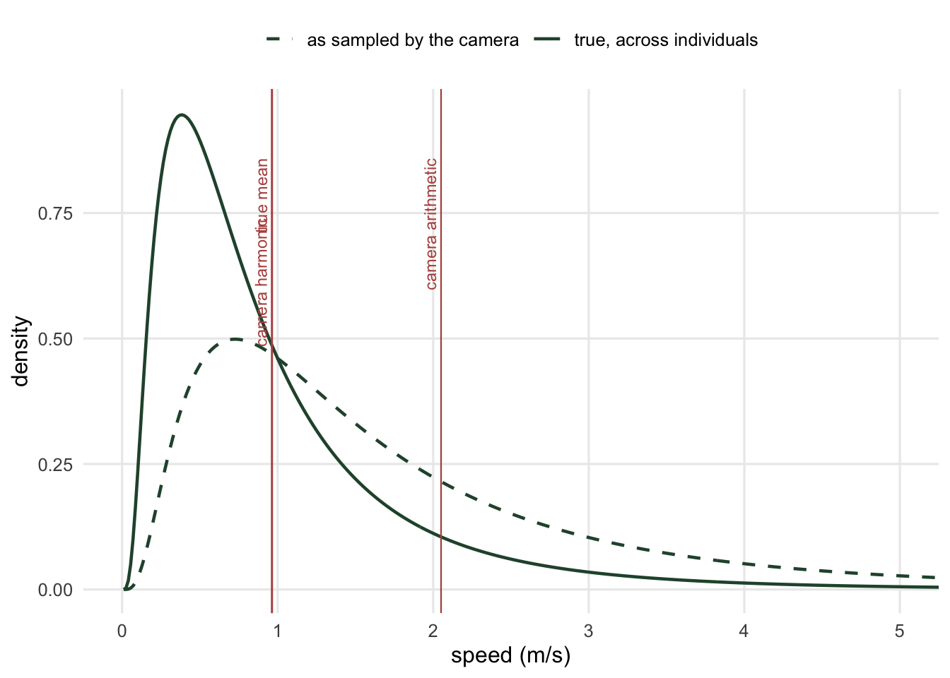
The dashed curve is not a different population. It is the same animals, weighted by how often they walk past a camera.
What it costs the density estimate
Push both speeds through the random encounter model and watch the density move.
rem_D <- function(y, t, v, r, theta) y * pi / (t * v * r * (2 + theta))
Dtrue <- n / A
rate <- length(obs) / Tt
out <- data.frame(
  speed_used = c("camera arithmetic mean", "camera harmonic mean"),
  v = c(mean(obs), 1 / mean(1 / obs)))
out$D_hat <- rem_D(length(obs), Tt, out$v, r, 2 * half)
out$ratio_to_truth <- out$D_hat / Dtrue
out
speed_used v D_hat ratio_to_truth
1 camera arithmetic mean 2.0505088 0.1769812 0.4719498
2 camera harmonic mean 0.9618642 0.3772897 1.0061058Using the obvious average of the camera’s own speed measurements loses 53 per cent of the population. Nothing in the fit complains: the encounter counts are the same, the speed sample is large, its standard error is small, and the answer is wrong by a factor of 2.1. This is what a bias with no diagnostic looks like, and the only defence is knowing the identity in advance.
One caveat on the identity: it corrects for the sampling, not for the measurement. If your speeds are noisy, that noise inflates the observed coefficient of variation and the harmonic mean of a noisy sample is dragged down by small values. The identity is exact for speeds measured exactly. Rowcliffe et al. (2016) handle this by fitting a parametric model to the observed speeds rather than taking a raw harmonic mean, which is the right move when the sample is small or the noise is large.
The other factor: how much of the day is spent moving
Every speed the camera measures comes from an animal that was moving, because a stationary animal produces no passage. So the harmonic mean above estimates \(v_{\text{active}}\), not \(v\). A deer that walks at 1 m/s for two hours a day and lies down for the other twenty-two has \(v_{\text{active}} = 1\) but \(v = 1/12\).
Rowcliffe et al. (2014) close the gap with an argument that is almost too neat. Records arrive at a rate proportional to the proportion of the population that is active, \(a(t)\), at time of day \(t\). So the density of record times is \(a(t)\) divided by its integral. If you are willing to assume that at the busiest moment of the day everyone is active, so that \(\max_t a(t) = 1\), then the integral is pinned down and the activity level falls out:
\[A = \frac{1}{2\pi}\int_0^{2\pi} a(t)\,\mathrm{d}t = \frac{1}{2\pi \max_t \hat{f}(t)}\]
where \(\hat{f}\) is a circular density fitted to the record times. Here is a crepuscular schedule and the estimator working on it. The kernel is von Mises, with its concentration chosen by leave-one-out likelihood cross-validation; the circular kernel machinery is covered in the activity overlap post.
vm <- function(x, mu, k) exp(k * cos(x - mu)) / (2 * pi * besselI(k, 0))
grid <- seq(0, 2 * pi, length.out = 2001)[-2001]
shape_raw <- function(x) 0.55 * vm(x, 1.4, 6) + 0.45 * vm(x, 4.3, 4)
gmax <- max(shape_raw(grid))
shape <- function(x) shape_raw(x) / gmax          # scaled so that max(shape) = 1
A_shape <- mean(shape(grid))                      # the activity level if the peak is 1

kern_f <- function(x, dat, k)
  vapply(x, function(z) mean(exp(k * cos(z - dat)) / (2 * pi * besselI(k, 0))), numeric(1))

lcv_k <- function(dat) {                          # leave-one-out likelihood CV
  m <- length(dat)
  nll <- function(lk) {
    k <- exp(lk)
    Cm <- outer(dat, dat, function(a, b) exp(k * cos(a - b)))
    diag(Cm) <- 0
    -sum(log(rowSums(Cm) / ((m - 1) * 2 * pi * besselI(k, 0))))
  }
  exp(optimise(nll, c(log(0.3), log(200)))$minimum)
}

set.seed(2602)
nrec <- 1200
tt <- (sample(grid, nrec, replace = TRUE, prob = shape(grid)) +
         runif(nrec, 0, 2 * pi / 2000)) %% (2 * pi)
k_hat <- lcv_k(tt)
A_hat <- 1 / (2 * pi * max(kern_f(grid, tt, k_hat)))
c(kappa_cv = k_hat, A_hat = A_hat, A_shape = A_shape, ratio = A_hat / A_shape)
kappa_cv A_hat A_shape ratio
41.4671885 0.3080587 0.3029394 1.0168985 The estimator recovers the activity level to within 2 per cent, and that residual has two parts. A kernel lowers the peak of a density and the peak sits in the denominator, so smoothing pushes \(\hat{A}\) high; that part always points the same way, and it gets worse fast if the kernel is too wide. Sampling noise moves the height of the fitted peak as well: in this sample it lifted the peak and offset most of the smoothing bias, and in another sample it can add to that bias or put \(\hat{A}\) below the truth.
     kappa     A_hat ratio_to_truth                       note
1  3.00000 0.5335572       1.761267             far too smooth
2 10.00000 0.3782579       1.248625                 too smooth
3 40.00000 0.3092049       1.020682                      close
4 41.46719 0.3080587       1.016899 chosen by cross-validation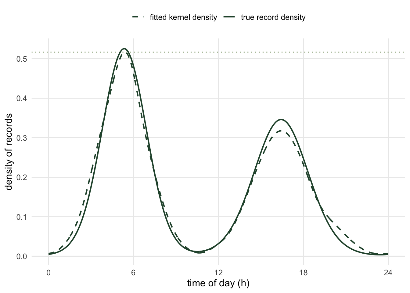
The assumption is doing all the work
Now the part that matters. Everything above assumed the peak is 1. Suppose it is not: suppose that even at dawn, only 70 per cent of the population is up and about. What does the camera see?
  peak_activity    true_A     A_hat    ratio
1           1.0 0.3029394 0.3080587 1.016899
2           0.7 0.2120576 0.3080587 1.452712
3           0.4 0.1211758 0.3080587 2.542246
Exactly the same records. The peak activity scales \(a(t)\) up and down, but the density of record times is \(a(t)\) divided by its own integral, and the scale factor cancels out of the ratio. The three worlds in that table are observationally identical to the activity estimator: same shape, same fit, same \(\hat{A}\), and, with the density raised to make up for the lower activity, even the same expected number of records at every hour. Only the truth differs, by a factor of 2.5 between the first row and the last.
So \(\hat{A}\) is not an estimate of the activity level in the way that a mean is an estimate of a mean. It is the activity level conditional on the peak being 1, and that condition is not testable with time-of-day data, no matter how many records you gather. Rowcliffe et al. (2014) state this openly, and it is a fair assumption for many species at their daily peak. It is not a fair assumption for a species with two behavioural classes on different schedules, or in a season when half the population is denning.
Notice what this does to the density estimate downstream. If the true peak is 0.7, then \(\hat{A}\) is 1.4 times too high, so \(\hat{v}\) is 1.4 times too high, so \(\hat{D}\) is 0.70 times the truth. Add the size-bias trap and a naive analyst has multiplied two errors in the same direction.
Where to go next
Both halves of \(v\) come from the same cameras that produced \(y\). That is convenient, and it is easy to read the wrong way: if the cameras sit somewhere the animals move faster than average, the speed is inflated and the encounter rate is inflated with it, but the density estimate divides the encounter rate by the speed, so the two errors pull it in opposite directions and tend to cancel. The checking post takes up a placement error that does not cancel, cameras put where the animals are denser. The alternative is to stop measuring speed altogether and read the geometry backwards, using how long animals stay in view instead of how fast they cross it. That is the staying time model, and it removes the speed measurement at the cost of a different one.
References
- Rowcliffe, Jansen, Kays, Kranstauber, Carbone 2016 Remote Sensing in Ecology and Conservation 2(2):84-94 (10.1002/rse2.17)
- Rowcliffe, Kays, Kranstauber, Carbone, Jansen 2014 Methods in Ecology and Evolution 5(11):1170-1179 (10.1111/2041-210X.12278)
- Rowcliffe, Field, Turvey, Carbone 2008 Journal of Applied Ecology 45(4):1228-1236 (10.1111/j.1365-2664.2008.01473.x)
- Rowcliffe, Carbone, Jansen, Kays, Kranstauber 2011 Methods in Ecology and Evolution 2(5):464-476 (10.1111/j.2041-210X.2011.00094.x)
- Palencia, Rowcliffe, Vicente, Acevedo 2021 Journal of Applied Ecology 58:1583-1592 (10.1111/1365-2664.13913)