---
title: "Activity patterns and temporal overlap"
description: "Camera-trap activity times as circular data: von Mises kernel density, the coefficient of overlap for temporal niche partitioning, and a bootstrap interval."
date: "2026-06-08 12:00"
date-modified: "2026-09-30"
categories: [R, circular statistics, camera traps, ecology tutorial, ggplot2]
image: thumbnail.png
image-alt: "Two activity curves on a single 24-hour axis, one peaking at midnight and one at dawn and dusk, with their overlap shaded grey beneath the lower of the two curves. The shaded area swells where the curves cross, near 04:00 and 20:00, and thins almost to nothing at midday."
---
*Corrected 30 September 2026: the post gave Ridout and Linkie's small-sample recommendation to the data-point estimator and swapped the published names Dhat1 and Dhat4; it now gives it to the grid estimator (their Dhat1), and it now says the camera bootstrap's coverage falls short of the control's only with the smaller number of cameras, not with both.*
*Updated 27 September 2026: a new section, Cameras, not detections, measures how far the detection bootstrap understates the interval when activity timing differs between cameras, and the paragraph that introduces the bootstrap now says when detections are the right unit to resample.*
*Corrected 25 September 2026: the sample-size caution in "What the overlap number hides" said the overlap estimator is biased upward when detections are few. Near complete overlap it runs low, and the section now measures both directions and points to the equivalency test.*
Camera traps record when animals are active, and time of day is circular: a detection at 23:30 and one at 00:30 are an hour apart, not twenty-three. Once times are wrapped onto the circle, two questions follow naturally. What does a species' daily activity look like, and how much do two species overlap in time, a common proxy for competition, predator avoidance or temporal niche partitioning. This post estimates activity curves with a circular kernel density and measures overlap with the coefficient of overlap, all in base R, and then is honest about how much that overlap number can be trusted.
## From clock time to angles
Map a time of day in hours to an angle by stretching the 24-hour day around the circle. Midnight sits at the top, noon at the bottom.
```{r}
#| label: setup
#| message: false
#| warning: false
#| code-fold: true
#| code-summary: "Setup: packages, colours and plot theme"
library(ggplot2)
library(grid)
te_forest <- "#275139"; te_paper <- "#f5f4ee"; te_ink <- "#16241d"
te_body <- "#2c3a31"; te_line <- "#dad9ca"; te_sage <- "#93a87f"; te_label <- "#46604a"
te_amber <- "#cda23f"; te_rust <- "#b5534e"; te_slate <- "#5d6b61"
theme_te <- function(base_size = 11) {
  theme_minimal(base_size = base_size) +
    theme(plot.title = element_text(colour = te_ink, face = "bold", size = rel(1.0)),
          plot.subtitle = element_text(colour = te_label, size = rel(0.85)),
          axis.title = element_text(colour = te_body), axis.text = element_text(colour = te_body),
          panel.grid.major = element_line(colour = te_line, linewidth = 0.3),
          panel.grid.minor = element_blank(),
          plot.background = element_rect(fill = "#f5f4ee", colour = NA),
          panel.background = element_rect(fill = "#f5f4ee", colour = NA), legend.position = "none")
}
# von Mises sampler for the synthetic detections
rvm <- function(n, mu, kappa) {
  out <- numeric(n); a <- 1 + sqrt(1 + 4 * kappa^2); b <- (a - sqrt(2 * a)) / (2 * kappa)
  r <- (1 + b^2) / (2 * b); i <- 0
  while (i < n) { u1 <- runif(1); z <- cos(pi * u1); f <- (1 + r * z) / (r + z); c1 <- kappa * (r - f); u2 <- runif(1)
    if (c1 * (2 - c1) - u2 > 0 || log(c1 / u2) + 1 - c1 >= 0) {
      u3 <- runif(1); i <- i + 1; out[i] <- (mu + sign(u3 - 0.5) * acos(f)) %% (2 * pi) } }
  out
}
rmix <- function(n, mus, kappas, w) { k <- sample(seq_along(mus), n, TRUE, w)
  vapply(seq_len(n), function(i) rvm(1, mus[k[i]], kappas[k[i]]), numeric(1)) }
clock24 <- function(h) {                       # a 24-hour clock face with midnight at top
  ang <- seq(0, 2 * pi, length.out = 200); circ <- data.frame(x = cos(ang), y = sin(ang))
  ticks <- seq(0, 2 * pi * 18 / 24, by = 2 * pi * 6 / 24)
  tk <- data.frame(x0 = 0.98 * sin(ticks), y0 = 0.98 * cos(ticks),
                   x1 = 1.06 * sin(ticks), y1 = 1.06 * cos(ticks))
  lab <- data.frame(x = 1.18 * sin(ticks), y = 1.18 * cos(ticks), lab = c("00", "06", "12", "18"))
  list(geom_path(data = circ, aes(x, y), colour = te_line, linewidth = 0.5),
       geom_segment(data = tk, aes(x = x0, y = y0, xend = x1, yend = y1), colour = te_sage, linewidth = 0.5),
       geom_text(data = lab, aes(x, y, label = lab), colour = te_label, size = 2.9),
       coord_fixed(xlim = c(-1.3, 1.3), ylim = c(-1.3, 1.3)), theme_void(),
       theme(plot.title = element_text(colour = te_ink, face = "bold", size = 11, hjust = 0.5),
             plot.background = element_rect(fill = "#f5f4ee", colour = NA)))
}
```
```{r}
#| label: times
hour2rad <- function(h) 2 * pi * h / 24
rad2hour <- function(r) (r %% (2 * pi)) * 24 / (2 * pi)

# two synthetic species: A nocturnal (one peak at midnight), B crepuscular (dawn and dusk peaks)
set.seed(4252)
A <- rvm(120, mu = hour2rad(0), kappa = 2)                                   # 120 detections
B <- rmix(100, mus = hour2rad(c(6, 18)), kappas = c(4, 4), w = c(0.5, 0.5))  # 100 detections
```
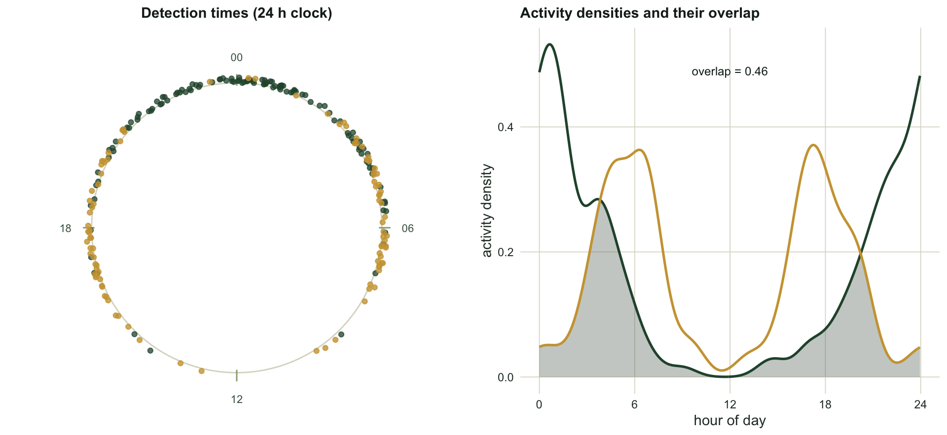
Species A is nocturnal, so its detections cluster around midnight with a mean resultant length of `r sprintf("%.2f", sqrt(mean(cos(A))^2 + mean(sin(A))^2))` and a mean activity time near `r sprintf("%02.0f:%02.0f", floor(rad2hour(atan2(mean(sin(A)), mean(cos(A))))), (rad2hour(atan2(mean(sin(A)), mean(cos(A)))) %% 1) * 60)`. Species B is crepuscular, with peaks at dawn and dusk, and here the tools from the earlier posts earn their keep: its mean resultant length is only `r sprintf("%.2f", sqrt(mean(cos(B))^2 + mean(sin(B))^2))`, because the two opposite peaks cancel. A single mean direction would be meaningless for B, and the Rayleigh test would call it uniform. The activity pattern is not a summary statistic; it is a whole curve, and that is what a density estimate provides.
## A circular kernel density
The circular analogue of a smoothed histogram places a small von Mises bump on each observation and averages them. The concentration of that bump is the bandwidth: a large concentration gives a wiggly curve that chases every detection, a small one gives a smooth curve that can wash out real peaks.
```{r}
#| label: kde
dvm  <- function(x, mu, kappa) exp(kappa * cos(x - mu)) / (2 * pi * besselI(kappa, 0))

ckde <- function(eval, data, kappa_bw) {           # von Mises kernel density
  sapply(eval, function(e) mean(dvm(e, data, kappa_bw)))
}

kappa_bw <- 20                                     # smoothing concentration (about a one-hour kernel)
grid <- seq(0, 2 * pi, length.out = 512)
fA <- ckde(grid, A, kappa_bw)
fB <- ckde(grid, B, kappa_bw)
```
## The coefficient of overlap
Temporal overlap between two activity curves is the area under the lower of the two densities: where both species are active, they overlap; where only one is, they do not. The coefficient of overlap runs from zero (no shared activity time) to one (identical activity). The natural estimator integrates the minimum of the two kernel densities over the circle (Ridout and Linkie 2009).
```{r}
#| label: overlap
overlap_D1 <- function(A, B, kappa_bw, ngrid = 512) {   # grid estimator, for small samples
  g <- seq(0, 2 * pi, length.out = ngrid + 1)[-(ngrid + 1)]; dg <- 2 * pi / ngrid
  sum(pmin(ckde(g, A, kappa_bw), ckde(g, B, kappa_bw))) * dg
}
overlap_D4 <- function(A, B, kappa_bw) {                # data-point estimator, for larger samples
  0.5 * (mean(pmin(1, ckde(A, B, kappa_bw) / ckde(A, A, kappa_bw))) +
         mean(pmin(1, ckde(B, A, kappa_bw) / ckde(B, B, kappa_bw))))
}

D1 <- overlap_D1(A, B, kappa_bw)
D4 <- overlap_D4(A, B, kappa_bw)
round(c(Dhat1 = D1, Dhat4 = D4), 3)
```
The grid estimator (Dhat1 in Ridout and Linkie, the one they recommend when the smaller sample is below about fifty) gives an overlap of `r sprintf("%.2f", D1)`, and the data-point estimator (their Dhat4, for larger samples) gives `r sprintf("%.2f", D4)`. The two agree closely here because both samples are reasonably large. That much shared activity time fits the picture: the nocturnal species is active through the dusk and dawn shoulders where the crepuscular species peaks.
```{r}
#| label: fig-activity
#| echo: false
#| fig-cap: "Left: detection times on a 24-hour clock, nocturnal species A in green clustered at midnight, crepuscular species B in amber at dawn and dusk. Right: the two kernel density estimates unrolled onto a linear day, with the shared area (the coefficient of overlap) shaded."
#| fig-alt: "Left panel is a 24-hour clock with green points bunched at the top near midnight and amber points at the six and eighteen o'clock positions. Right panel plots two activity density curves against hour of day; the green curve peaks at midnight, the amber curve has two peaks at dawn and dusk, and the overlap between them is shaded grey."
#| fig-width: 10
#| fig-height: 4.6
jit <- function(x) 1 + (seq_along(x) %% 7) * 0.006
dA <- data.frame(x = jit(A) * sin(A), y = jit(A) * cos(A))
dB <- data.frame(x = jit(B) * sin(B), y = jit(B) * cos(B))
sp_cols <- c("species A (nocturnal)" = te_forest, "species B (crepuscular)" = te_amber)
sp_key <- list(scale_colour_manual(values = sp_cols, name = NULL),
theme(legend.position = "top",
legend.text = element_text(colour = te_body, size = 8.5)))
pClock <- ggplot() + clock24() +
geom_point(data = dA, aes(x, y, colour = names(sp_cols)[1]), size = 1.5, alpha = 0.75) +
geom_point(data = dB, aes(x, y, colour = names(sp_cols)[2]), size = 1.5, alpha = 0.8) +
guides(colour = guide_legend(override.aes = list(size = 2.2, alpha = 1))) +
sp_key +
ggtitle("Detection times (24 h clock)")
hh <- rad2hour(grid); ord <- order(hh)
dens <- data.frame(hour = hh[ord], fa = fA[ord], fb = fB[ord])
dens$lo <- pmin(dens$fa, dens$fb)
pDens <- ggplot(dens, aes(hour)) +
geom_ribbon(aes(ymin = 0, ymax = lo), fill = te_slate, alpha = 0.35) +
geom_line(aes(y = fa, colour = names(sp_cols)[1]), linewidth = 0.9) +
geom_line(aes(y = fb, colour = names(sp_cols)[2]), linewidth = 0.9) +
annotate("text", x = 12, y = max(dens$fa) * 0.92, label = sprintf("overlap = %.2f", D1),
colour = te_ink, size = 3.2) +
scale_x_continuous(breaks = c(0, 6, 12, 18, 24), limits = c(0, 24)) +
labs(title = "Activity densities and their overlap", x = "hour of day", y = "activity density") +
theme_te(11) + sp_key
grid.newpage(); pushViewport(viewport(layout = grid.layout(1, 2)))
print(pClock, vp = viewport(layout.pos.row = 1, layout.pos.col = 1))
print(pDens, vp = viewport(layout.pos.row = 1, layout.pos.col = 2))
```
## A bootstrap interval
A single overlap number needs an interval. The synthetic detections here are independent draws, so the activity times can serve as the sampling unit: resample detections within each species with replacement, recompute the overlap, and take the percentiles of the bootstrap distribution. Real detections arrive camera by camera, and the section after this one measures when that matters.
```{r}
#| label: bootstrap
set.seed(11)
Dboot <- replicate(2000, {
  a <- sample(A, replace = TRUE); b <- sample(B, replace = TRUE)
  overlap_D1(a, b, kappa_bw, ngrid = 256)
})
ci <- quantile(Dboot, c(0.025, 0.975))
round(c(estimate = D1, lower = ci[[1]], upper = ci[[2]]), 3)
```
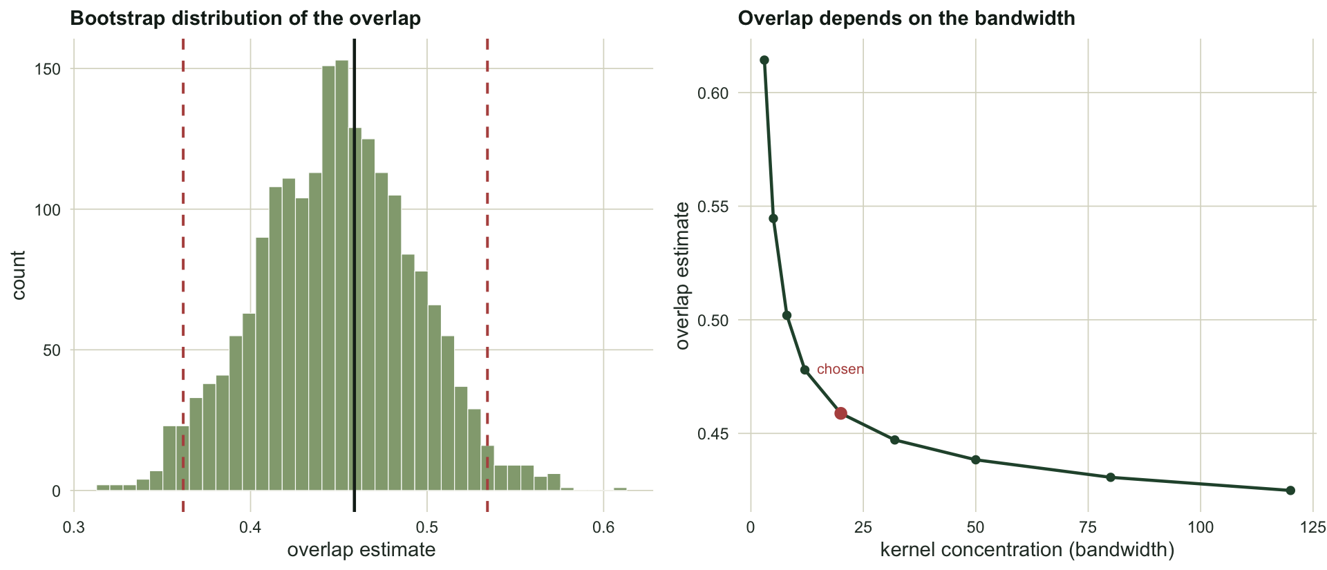
The bootstrap gives a 95 per cent interval of `r sprintf("%.2f", ci[[1]])` to `r sprintf("%.2f", ci[[2]])`, a width of `r sprintf("%.2f", ci[[2]] - ci[[1]])`. That is wide. Overlap coefficients are noisy, and reporting the point estimate alone would overstate what a couple of hundred detections can pin down.
## Cameras, not detections
The bootstrap above treats every detection as an independent draw. Camera-trap detections arrive in batches, one batch per camera, and if the timing of activity differs from camera to camera (a cooler valley, a clock left on summer time), every detection from one camera carries the same shift. The chunk below spreads this post's two species over cameras with uneven detection counts (negative binomial with size 1, totals averaging 120 and 100 as in the `times` chunk) and moves each camera's detections by a normal shift with standard deviation `sd_cam` radians, either the same shift for both species or an independent one. The shift sizes and camera numbers are assumptions chosen to span a range, not values taken from data. Each simulated study is scored with the detection bootstrap of the previous section and with a camera bootstrap that resamples whole cameras, the principle of "Clusters, not rows" in [Bootstrapping dependent data: blocks and clusters](../bootstrapping-dependent-data/). For speed, detections are binned to 128 bins and smoothed with a kernel matrix at this post's bandwidth; resampling detections and then binning is the same as a multinomial draw on the bin counts, and the `stopifnot()` checks the binned estimator against `overlap_D1()` on this post's own A and B.
```{r}
#| label: camera-bootstrap
cam_G <- 128
cam_mid <- (seq_len(cam_G) - 0.5) * 2 * pi / cam_G
cam_K <- outer(cam_mid, cam_mid, dvm, kappa = kappa_bw)         # kernel matrix, same bandwidth
cam_bin <- function(x) tabulate(floor((x %% (2 * pi)) / (2 * pi) * cam_G) + 1, cam_G)
cam_ovl <- function(ca, cb) {                                   # one overlap per column of bin counts
  colSums(pmin(cam_K %*% sweep(ca, 2, colSums(ca), "/"),
               cam_K %*% sweep(cb, 2, colSums(cb), "/"))) * 2 * pi / cam_G
}
stopifnot(abs(cam_ovl(cbind(cam_bin(A)), cbind(cam_bin(B))) - D1) < 0.005)

cam_study <- function(n_cam, sd_cam, shared, n_boot = 199) {
  sA <- rnorm(n_cam, 0, sd_cam); sB <- if (shared) sA else rnorm(n_cam, 0, sd_cam)
  nA <- rnbinom(n_cam, size = 1, mu = 120 / n_cam); nB <- rnbinom(n_cam, size = 1, mu = 100 / n_cam)
  MA <- sapply(seq_len(n_cam), function(k) cam_bin(rvm(nA[k], hour2rad(0) + sA[k], 2)))
  MB <- sapply(seq_len(n_cam), function(k)
    cam_bin(rmix(nB[k], hour2rad(c(6, 18)) + sB[k], c(4, 4), c(0.5, 0.5))))
  ca <- rowSums(MA); cb <- rowSums(MB)
  det_bt <- cam_ovl(rmultinom(n_boot, sum(ca), ca), rmultinom(n_boot, sum(cb), cb))
  W <- rmultinom(n_boot, n_cam, rep(1, n_cam))                  # times each camera is drawn
  lost <- colSums(MA %*% W) == 0 | colSums(MB %*% W) == 0
  while (any(lost)) {                                           # redraw resamples that lose a species
    W[, lost] <- rmultinom(sum(lost), n_cam, rep(1, n_cam))
    lost <- colSums(MA %*% W) == 0 | colSums(MB %*% W) == 0
  }
  cam_bt <- cam_ovl(MA %*% W, MB %*% W)
  c(est = cam_ovl(cbind(ca), cbind(cb))[[1]], det_se = sd(det_bt), cam_se = sd(cam_bt),
    eff = sum(nA)^2 / sum(nA^2),                                # effective number of cameras, species A
    det_lo = quantile(det_bt, 0.025, names = FALSE), det_hi = quantile(det_bt, 0.975, names = FALSE),
    cam_lo = quantile(cam_bt, 0.025, names = FALSE), cam_hi = quantile(cam_bt, 0.975, names = FALSE))
}

cam_R <- 1500                                                   # simulated studies per scenario
cam_scen <- data.frame(cameras = c(25, 25, 25, 25, 12), sd_cam = c(0, 0.3, 0.6, 0.6, 0.6),
                       shift = c("none", "shared", "shared", "independent", "shared"))
set.seed(4253)
cam_out <- t(sapply(seq_len(nrow(cam_scen)), function(i) {
  r <- replicate(cam_R, cam_study(cam_scen$cameras[i], cam_scen$sd_cam[i],
                                  cam_scen$shift[i] != "independent"))
  m <- mean(r["est", ]); s <- sd(r["est", ])
  c(mean_overlap = m, det_ratio = mean(r["det_se", ]) / s, cam_ratio = mean(r["cam_se", ]) / s,
    det_cover = mean(r["det_lo", ] <= m & r["det_hi", ] >= m),
    cam_cover = mean(r["cam_lo", ] <= m & r["cam_hi", ] >= m), eff_cameras = mean(r["eff", ]))
}))
cam_mcz <- function(ratio) (1 - ratio) / (ratio / sqrt(2 * (cam_R - 1)))   # distance below 1 in MC errors
cam_covz <- function(p0, p) (p0 - p) / sqrt((p0 * (1 - p0) + p * (1 - p)) / cam_R)  # coverage gap in MC errors
cbind(cam_scen, shift_hours = round(cam_scen$sd_cam * 24 / (2 * pi), 1), round(cam_out, 2))
```
A ratio is the average bootstrap standard error divided by the standard deviation of the overlap estimate across the `r cam_R` studies, so 1 means the bootstrap reports the real spread. That standard deviation carries a Monte Carlo error of about `r sprintf("%.3f", 1 / sqrt(2 * (cam_R - 1)))` in relative terms, and a coverage near 0.95 about `r sprintf("%.3f", sqrt(0.95 * 0.05 / cam_R))`. Coverage here is the share of 95 per cent percentile intervals that contain the mean estimate across studies, not the true overlap, so it scores the width and placement of the interval and leaves the estimator's own bias to the next section.
Uneven counts alone barely change the ratio: with no shift, the detection bootstrap's ratio is `r sprintf("%.2f", cam_out[1, "det_ratio"])` and the camera bootstrap's `r sprintf("%.2f", cam_out[1, "cam_ratio"])`, `r sprintf("%.1f", cam_mcz(cam_out[1, "det_ratio"]))` and `r sprintf("%.1f", cam_mcz(cam_out[1, "cam_ratio"]))` Monte Carlo errors below 1. This control row is also the yardstick for coverage: even here the percentile intervals cover the mean estimate in `r sprintf("%.2f", cam_out[1, "det_cover"])` and `r sprintf("%.2f", cam_out[1, "cam_cover"])` of studies, not 0.95. With a shared shift of `r sprintf("%.1f", 0.3 * 24 / (2 * pi))` hours across 25 cameras the detection bootstrap reports `r sprintf("%.2f", cam_out[2, "det_ratio"])` of the real spread, `r sprintf("%.1f", cam_mcz(cam_out[2, "det_ratio"]))` Monte Carlo errors below 1 but only a little below the control row, against `r sprintf("%.2f", cam_out[2, "cam_ratio"])` (`r sprintf("%.1f", cam_mcz(cam_out[2, "cam_ratio"]))` errors) for the camera bootstrap, while coverage of `r sprintf("%.2f", cam_out[2, "det_cover"])` and `r sprintf("%.2f", cam_out[2, "cam_cover"])` still matches the control. At `r sprintf("%.1f", 0.6 * 24 / (2 * pi))` hours the detection bootstrap falls well behind: it reports `r sprintf("%.2f", cam_out[3, "det_ratio"])` of the real spread with 25 cameras and `r sprintf("%.2f", cam_out[5, "det_ratio"])` with 12, and its intervals cover the mean estimate in `r sprintf("%.2f", cam_out[3, "det_cover"])` and `r sprintf("%.2f", cam_out[5, "det_cover"])` of studies. Resampling cameras gives ratios of `r sprintf("%.2f", cam_out[3, "cam_ratio"])` and `r sprintf("%.2f", cam_out[5, "cam_ratio"])`, with coverage `r sprintf("%.2f", cam_out[3, "cam_cover"])` and `r sprintf("%.2f", cam_out[5, "cam_cover"])`. Independent shifts for the two species give ratios of `r sprintf("%.2f", cam_out[4, "det_ratio"])` for detections against `r sprintf("%.2f", cam_out[4, "cam_ratio"])` for cameras.
The camera bootstrap narrows the gap without closing it, and how much it closes depends on the number of cameras. At `r sprintf("%.1f", 0.6 * 24 / (2 * pi))` hours its ratio sits `r sprintf("%.1f", cam_mcz(cam_out[3, "cam_ratio"]))` Monte Carlo errors below 1 with 25 cameras and `r sprintf("%.1f", cam_mcz(cam_out[5, "cam_ratio"]))` with 12, and its coverage is `r sprintf("%.2f", cam_out[3, "cam_cover"])` with 25 cameras and `r sprintf("%.2f", cam_out[5, "cam_cover"])` with 12, against the control's `r sprintf("%.2f", cam_out[1, "cam_cover"])`, differences of `r sprintf("%.1f", cam_covz(cam_out[1, "cam_cover"], cam_out[3, "cam_cover"]))` and `r sprintf("%.1f", cam_covz(cam_out[1, "cam_cover"], cam_out[5, "cam_cover"]))` Monte Carlo errors: no clear shortfall with 25 cameras, a clear one with 12. This is the few-clusters problem. With negative binomial counts the detections are spread unevenly over the cameras, so the pooled curve rests on fewer cameras than were set out: the effective number for species A, the squared total count over the sum of squared camera counts, averages `r sprintf("%.1f", cam_out[1, "eff_cameras"])` of 25 and `r sprintf("%.1f", cam_out[5, "eff_cameras"])` of 12, and a bootstrap that resamples so few units runs short. The cluster bootstrap in [Bootstrapping dependent data: blocks and clusters](../bootstrapping-dependent-data/) does well because twenty equal sites give plenty of units to resample.
The shift also changes what is being estimated. The pooled detections follow a mixture of the camera curves, each weighted by that camera's share of the detections, and the mean overlap across studies rises from `r sprintf("%.2f", cam_out[1, "mean_overlap"])` with no shift to `r sprintf("%.2f", cam_out[3, "mean_overlap"])` at `r sprintf("%.1f", 0.6 * 24 / (2 * pi))` hours with 25 cameras. Resampling cameras widens the interval around that pooled number; it does not remove the shift from the number. With real data, keep the camera identifier on every detection: the camera bootstrap needs nothing else, though with few cameras, or few that carry most of the detections, it still runs short.
## What the overlap number hides
Two cautions travel with any overlap estimate, and both are choices rather than facts about the animals. The first is the bandwidth. The same data give a range of answers depending on how much the densities are smoothed:
```{r}
#| label: bandwidth
sapply(c(5, 10, 20, 40, 80), function(k) round(overlap_D1(A, B, k), 3))
```
Smoothing harder, with a smaller kernel concentration, inflates the overlap, because two broad curves share more area than two sharp ones. The estimate swings from about `r sprintf("%.2f", overlap_D1(A, B, 80))` to `r sprintf("%.2f", overlap_D1(A, B, 5))` across sensible bandwidths, and there is no bandwidth that is objectively correct.
```{r}
#| label: same-activity
# sample size: 200 studies of two species with identical activity (species A's curve),
# 30 detections each, scored with the same two estimators and bandwidth as above
set.seed(530)
same_act <- replicate(200, {
  a30 <- rvm(30, mu = hour2rad(0), kappa = 2); b30 <- rvm(30, mu = hour2rad(0), kappa = 2)
  c(Dhat4 = overlap_D4(a30, b30, kappa_bw), Dhat1 = overlap_D1(a30, b30, kappa_bw, ngrid = 256))
})
round(rowMeans(same_act), 3)
# the same identical pair at this post's own sample sizes, 120 and 100 detections
set.seed(531)
same_own <- replicate(200, {
  a_own <- rvm(120, mu = hour2rad(0), kappa = 2); b_own <- rvm(100, mu = hour2rad(0), kappa = 2)
  c(Dhat4 = overlap_D4(a_own, b_own, kappa_bw), Dhat1 = overlap_D1(a_own, b_own, kappa_bw, ngrid = 256))
})
round(rowMeans(same_own), 3)
```
The second caution is sample size, and it pulls both ways. Smoothing draws the two estimated curves together and biases the overlap up; sampling noise makes them differ where the true curves agree and pulls it down. Two species with identical activity and 30 detections each score `r sprintf("%.2f", mean(same_act["Dhat4", ]))` with the data-point estimator and `r sprintf("%.2f", mean(same_act["Dhat1", ]))` with the grid estimator, averaged over 200 simulated studies, well short of one, and still only `r sprintf("%.2f", mean(same_own["Dhat4", ]))` and `r sprintf("%.2f", mean(same_own["Dhat1", ]))` at this post's own sample sizes of 120 and 100. Whether the data are compatible with complete overlap is therefore a question for the equivalency test of [Niche equivalency and similarity tests](../niche-equivalency-and-similarity-tests/), which pools the detections and reshuffles the species labels, so its null distribution carries the same shortfall. A percentile bootstrap interval cannot answer it: each resample draws the two species from different detections, so every bootstrap overlap falls below one. A test that does not reject is not evidence of complete overlap either; it may only mean too few detections to see a difference.
```{r}
#| label: fig-uncertainty
#| echo: false
#| fig-cap: "Left: the bootstrap distribution of the overlap estimate, with the point estimate (solid) and the 95 per cent interval (dashed). Right: the same overlap estimate as a function of the smoothing bandwidth; harder smoothing (smaller concentration) inflates the overlap, and no single value is objectively right."
#| fig-alt: "Left panel is a histogram of bootstrap overlap estimates, with a solid line at the point estimate and dashed lines marking the 95 per cent interval. Right panel plots the overlap estimate against kernel concentration, with the chosen bandwidth marked."
#| fig-width: 10
#| fig-height: 4.3
dboot <- data.frame(D = Dboot)
pBoot <- ggplot(dboot, aes(D)) +
geom_histogram(bins = 40, fill = te_sage, colour = "white", linewidth = 0.2) +
geom_vline(xintercept = D1, colour = te_ink, linewidth = 0.8) +
geom_vline(xintercept = ci, colour = te_rust, linetype = "dashed", linewidth = 0.7) +
labs(title = "Bootstrap distribution of the overlap", x = "overlap estimate", y = "count") +
theme_te(11)
kseq <- c(3, 5, 8, 12, 20, 32, 50, 80, 120)
bw_curve <- data.frame(kappa_bw = kseq, D = sapply(kseq, function(k) overlap_D1(A, B, k)))
pBW <- ggplot(bw_curve, aes(kappa_bw, D)) +
geom_line(colour = te_forest, linewidth = 0.8) + geom_point(colour = te_forest, size = 1.7) +
geom_point(data = subset(bw_curve, kappa_bw == 20), colour = te_rust, size = 2.6) +
annotate("text", x = 20, y = bw_curve$D[bw_curve$kappa_bw == 20] + 0.02, label = "chosen", colour = te_rust, size = 2.8) +
labs(title = "Overlap depends on the bandwidth", x = "kernel concentration (bandwidth)", y = "overlap estimate") +
theme_te(11)
grid.newpage(); pushViewport(viewport(layout = grid.layout(1, 2)))
print(pBoot, vp = viewport(layout.pos.row = 1, layout.pos.col = 1))
print(pBW, vp = viewport(layout.pos.row = 1, layout.pos.col = 2))
```
The checking post that closes this series simulates the upward, smoothing half of that bias against a known truth, with a bandwidth that tightens as the sample grows. The short version: an overlap coefficient is a useful, comparable summary, but it is a smoothed estimate with a real bias and a wide interval, not a precise measurement of shared time.
## References
Batschelet E 1981 Circular Statistics in Biology. Academic Press. ISBN 978-0-12-081050-5.
Fisher NI 1993 Statistical Analysis of Circular Data. Cambridge University Press. ISBN 978-0-521-35018-1.
Pewsey A, Neuhauser M, Ruxton GD 2013 Circular Statistics in R. Oxford University Press. ISBN 978-0-19-967113-7.
Ridout MS, Linkie M 2009 Journal of Agricultural, Biological, and Environmental Statistics 14(3):322-337 (10.1198/jabes.2009.08038).
Linkie M, Ridout MS 2011 Journal of Zoology 284(3):224-229 (10.1111/j.1469-7998.2011.00801.x).
Rowcliffe JM, Kays R, Kranstauber B, Carbone C, Jansen PA 2014 Methods in Ecology and Evolution 5(11):1170-1179 (10.1111/2041-210X.12278).
Taylor CC 2008 Computational Statistics and Data Analysis 52(7):3493-3500 (10.1016/j.csda.2007.11.003).
## Related tutorials
- [Circular data and the von Mises distribution](../circular-data-and-von-mises/)
- [Testing for circular uniformity](../testing-for-circular-uniformity/)
- [Checking a circular analysis](../checking-a-circular-analysis/)
- [Measuring animal speed from camera traps](../animal-speed-from-camera-traps/)