---
title: "Checking a circular analysis"
description: "Mean direction, concentration, uniformity verdicts and the overlap coefficient are decisions in disguise: what circular summaries hide, and how to report them."
date: "2026-06-08 13:00"
date-modified: "2026-09-30"
categories: [R, circular statistics, model checking, ecology tutorial, ggplot2]
image: thumbnail.png
image-alt: "A single panel line chart of an estimate against sample size from 10 to 100, with a grey truth line at 2.00. The raw series starts near 2.54 and falls steadily to about 2.04, staying above the truth line throughout, while the bias-corrected series starts just below it at 1.95 and stays within 0.01 of 2.00 from sample size 15 on."
---
*Corrected 30 September 2026: the overlap section said Ridout and Linkie recommend the data-point estimator for small samples; they recommend the grid estimator for small samples, and the text now says so and notes that the labels in this post's code are reversed relative to theirs.*
The three preceding posts each ended on a warning, and this one collects them. A circular analysis produces clean-looking numbers, a mean direction, a concentration, a p-value for uniformity, a coefficient of overlap, and every one of them depends on an assumption or a tuning choice that the number itself does not show. Report the number alone and you report a decision as though it were a fact. This post takes each summary in turn, in base R, and asks what it hides and how to check it.
```{r}
#| label: setup
#| message: false
#| warning: false
#| code-fold: true
#| code-summary: "Setup: packages, colours and plot theme"
library(ggplot2)
library(grid)
te_forest <- "#275139"; te_paper <- "#f5f4ee"; te_ink <- "#16241d"
te_body <- "#2c3a31"; te_line <- "#dad9ca"; te_sage <- "#93a87f"; te_label <- "#46604a"
te_amber <- "#cda23f"; te_rust <- "#b5534e"; te_slate <- "#5d6b61"
theme_te <- function(base_size = 11) {
  theme_minimal(base_size = base_size) +
    theme(plot.title = element_text(colour = te_ink, face = "bold", size = rel(1.0)),
          plot.subtitle = element_text(colour = te_label, size = rel(0.85)),
          axis.title = element_text(colour = te_body), axis.text = element_text(colour = te_body),
          panel.grid.major = element_line(colour = te_line, linewidth = 0.3),
          panel.grid.minor = element_blank(),
          plot.background = element_rect(fill = "#f5f4ee", colour = NA),
          panel.background = element_rect(fill = "#f5f4ee", colour = NA), legend.position = "none")
}
circ_mean <- function(t) atan2(mean(sin(t)), mean(cos(t)))
circ_R    <- function(t) sqrt(mean(cos(t))^2 + mean(sin(t))^2)
A_kappa   <- function(k) besselI(k, 1) / besselI(k, 0)
kappa_mle <- function(R) if (R < 1e-8) 0 else if (R > 0.999999) Inf else uniroot(function(k) A_kappa(k) - R, c(1e-6, 700))$root
kappa_bc  <- function(k, n) { if (!is.finite(k)) return(k); if (k < 2) return(max(k - 2 / (n * k), 0)); (n - 1)^3 * k / (n^3 + n) }
dvm <- function(x, mu, k) exp(k * cos(x - mu)) / (2 * pi * besselI(k, 0))
rvm <- function(n, mu, kappa) {
  out <- numeric(n); a <- 1 + sqrt(1 + 4 * kappa^2); b <- (a - sqrt(2 * a)) / (2 * kappa)
  r <- (1 + b^2) / (2 * b); i <- 0
  while (i < n) { u1 <- runif(1); z <- cos(pi * u1); f <- (1 + r * z) / (r + z); c1 <- kappa * (r - f); u2 <- runif(1)
    if (c1 * (2 - c1) - u2 > 0 || log(c1 / u2) + 1 - c1 >= 0) {
      u3 <- runif(1); i <- i + 1; out[i] <- (mu + sign(u3 - 0.5) * acos(f)) %% (2 * pi) } }
  out
}
raxial <- function(n, mu, kappa) { s <- rvm(n, mu, kappa); fl <- runif(n) < 0.5; s[fl] <- (s[fl] + pi) %% (2 * pi); s }
rmix <- function(n, mus, kappas, w) { k <- sample(seq_along(mus), n, TRUE, w)
  vapply(seq_len(n), function(i) rvm(1, mus[k[i]], kappas[k[i]]), numeric(1)) }
rayleigh_Z <- function(th) length(th) * circ_R(th)^2
rao_U <- function(th) { n <- length(th); a <- sort(th %% (2 * pi)); g <- c(diff(a), 2 * pi - (a[n] - a[1])); 0.5 * sum(abs(g - 2 * pi / n)) }
kuiper_V <- function(th) { n <- length(th); u <- sort((th %% (2 * pi)) / (2 * pi)); max((1:n) / n - u) + max(u - (0:(n - 1)) / n) }
watson_U2 <- function(th) { n <- length(th); u <- sort((th %% (2 * pi)) / (2 * pi)); ub <- mean(u); i <- 1:n; sum((u - (2 * i - 1) / (2 * n))^2) + 1 / (12 * n) - n * (ub - 0.5)^2 }
allstats <- function(th) c(Rayleigh = rayleigh_Z(th), Rao = rao_U(th), Kuiper = kuiper_V(th), Watson = watson_U2(th))
ckde <- function(eval, data, kbw) sapply(eval, function(e) mean(dvm(e, data, kbw)))
```
## The mean direction can be a mirage
The mean direction and the mean resultant length come as a pair, and the resultant length is the warning label. When it is close to zero, the mean direction is not a weak preference, it is meaningless: a two-way or multi-way pattern produces a near-zero resultant no matter how tightly the sub-groups cluster. Take a strongly bimodal sample, animals moving along an axis, and resample it to see how stable its mean direction is.
```{r}
#| label: mean-dir
set.seed(4253)
unimodal <- rvm(60, mu = pi / 2, kappa = 2)   # one preferred direction
bimodal  <- raxial(60, mu = pi / 2, kappa = 4) # a two-way axis

boot_dir <- function(x, B = 2000) { set.seed(7); replicate(B, circ_mean(sample(x, replace = TRUE)) %% (2 * pi)) }
sd_deg <- function(ang) sqrt(-2 * log(circ_R(ang))) * 180 / pi
du <- boot_dir(unimodal); db <- boot_dir(bimodal)
c(unimodal_Rbar = circ_R(unimodal), bimodal_Rbar = circ_R(bimodal),
  unimodal_dir_SD = sd_deg(du), bimodal_dir_SD = sd_deg(db))
```
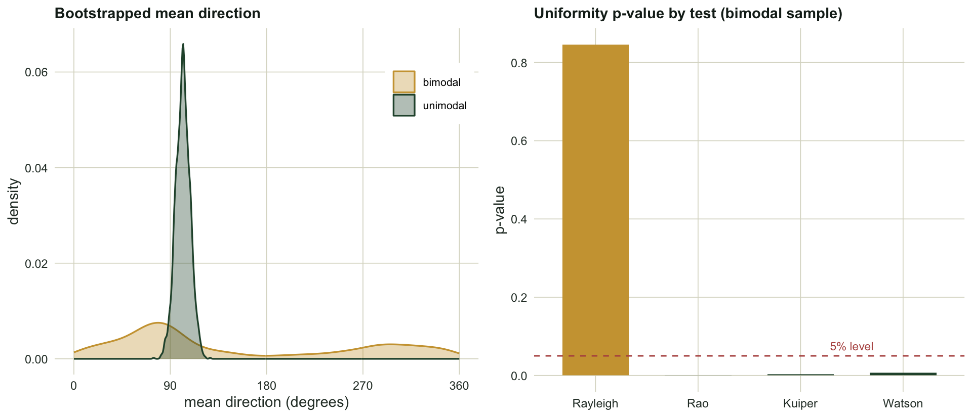
The unimodal sample has a resultant length of `r sprintf("%.2f", circ_R(unimodal))`, and its mean direction is stable: across bootstrap resamples the direction varies by a circular standard deviation of only `r sprintf("%.0f", sd_deg(du))` degrees. The bimodal sample has a resultant length of `r sprintf("%.2f", circ_R(bimodal))`, near zero, and its mean direction is worthless: it wanders across `r sprintf("%.0f", sd_deg(db))` degrees between resamples, so there is no stable direction to report. The lesson from the first post, stated as a check: never report a mean direction without its resultant length, and treat a small resultant not as a weak signal but as a sign that a single direction is the wrong summary.
## The uniformity verdict depends on the test
The same bimodal sample exposes the second warning. Whether it counts as evidence of a preferred direction depends entirely on which uniformity test you run.
```{r}
#| label: test-choice
set.seed(808)
null60 <- t(replicate(5000, allstats(runif(60, 0, 2 * pi))))
pvals <- sapply(1:4, function(j) mean(null60[, j] >= allstats(bimodal)[j]))
names(pvals) <- c("Rayleigh", "Rao", "Kuiper", "Watson")
round(pvals, 4)
```
The Rayleigh test returns a p-value of `r sprintf("%.2f", pvals[1])` and finds nothing, because the near-zero resultant it is built on carries no signal. The omnibus tests, Rao, Kuiper and Watson, ask a different question of the same sample, and the difference between the four p-values is not sampling noise but the question each statistic encodes. The check here is to choose the test before seeing the data, guided by the biology: if two-way or multi-way patterns are plausible, an omnibus test is required and the Rayleigh test alone will mislead. This is exactly the shift recent ecological work recommends (Landler, Ruxton and Malkemper 2018, 2019).
```{r}
#| label: fig-verdict
#| echo: false
#| fig-cap: "Left: bootstrap distributions of the mean direction. The unimodal sample (green) concentrates tightly; the bimodal sample (amber) spreads right round the circle with only a weak peak, so its mean direction is meaningless. Right: uniformity p-values for the bimodal sample. The Rayleigh test sits above the five per cent line and fails to reject."
#| fig-alt: "Left panel shows two density curves of bootstrap mean directions in degrees: a tall narrow green peak and a low, broad amber distribution with a weak peak near eighty degrees and some mass at every angle. Right panel is a bar chart of four p-values with a dashed line at 0.05; the Rayleigh bar rises above the line."
#| fig-width: 10
#| fig-height: 4.3
dird <- rbind(data.frame(deg = du * 180 / pi, grp = "unimodal"),
data.frame(deg = db * 180 / pi, grp = "bimodal"))
pDir <- ggplot(dird, aes(deg, fill = grp, colour = grp)) +
geom_density(alpha = 0.35, adjust = 0.6, linewidth = 0.6) +
scale_fill_manual(values = c(unimodal = te_forest, bimodal = te_amber)) +
scale_colour_manual(values = c(unimodal = te_forest, bimodal = te_amber)) +
scale_x_continuous(breaks = c(0, 90, 180, 270, 360), limits = c(0, 360)) +
labs(title = "Bootstrapped mean direction", x = "mean direction (degrees)", y = "density") +
theme_te(11) + theme(legend.position = "inside", legend.position.inside = c(0.99, 0.9), legend.justification = c(1, 1),
legend.title = element_blank(), legend.text = element_text(size = 8),
legend.background = element_rect(fill = "white", colour = NA))
pbar <- data.frame(test = factor(names(pvals), levels = names(pvals)), p = as.numeric(pvals))
pP <- ggplot(pbar, aes(test, p, fill = p > 0.05)) +
geom_col(width = 0.65) +
geom_hline(yintercept = 0.05, linetype = "dashed", colour = te_rust) +
annotate("text", x = 3.5, y = 0.075, label = "5% level", colour = te_rust, size = 3) +
scale_fill_manual(values = c(`TRUE` = te_amber, `FALSE` = te_forest)) +
labs(title = "Uniformity p-value by test (bimodal sample)", x = NULL, y = "p-value") +
theme_te(11)
grid.newpage(); pushViewport(viewport(layout = grid.layout(1, 2)))
print(pDir, vp = viewport(layout.pos.row = 1, layout.pos.col = 1))
print(pP, vp = viewport(layout.pos.row = 1, layout.pos.col = 2))
```
## The concentration is biased upward in small samples
The concentration parameter kappa has a quieter problem: its maximum-likelihood estimate is biased, and the bias is large exactly when samples are small, which is when ecologists most want a number. Simulate from a known concentration and watch the estimate.
```{r}
#| label: kappa-bias
kappa_true <- 2
kbias <- do.call(rbind, lapply(c(10, 15, 25, 50, 100), function(n) {
  set.seed(500 + n)
  est <- t(replicate(2500, { x <- rvm(n, 0, kappa_true); kh <- kappa_mle(circ_R(x)); c(kh, kappa_bc(kh, n)) }))
  data.frame(n = n, mle = mean(est[is.finite(est[, 1]), 1]), corrected = mean(est[is.finite(est[, 2]), 2]))
}))
round(kbias, 2)
```
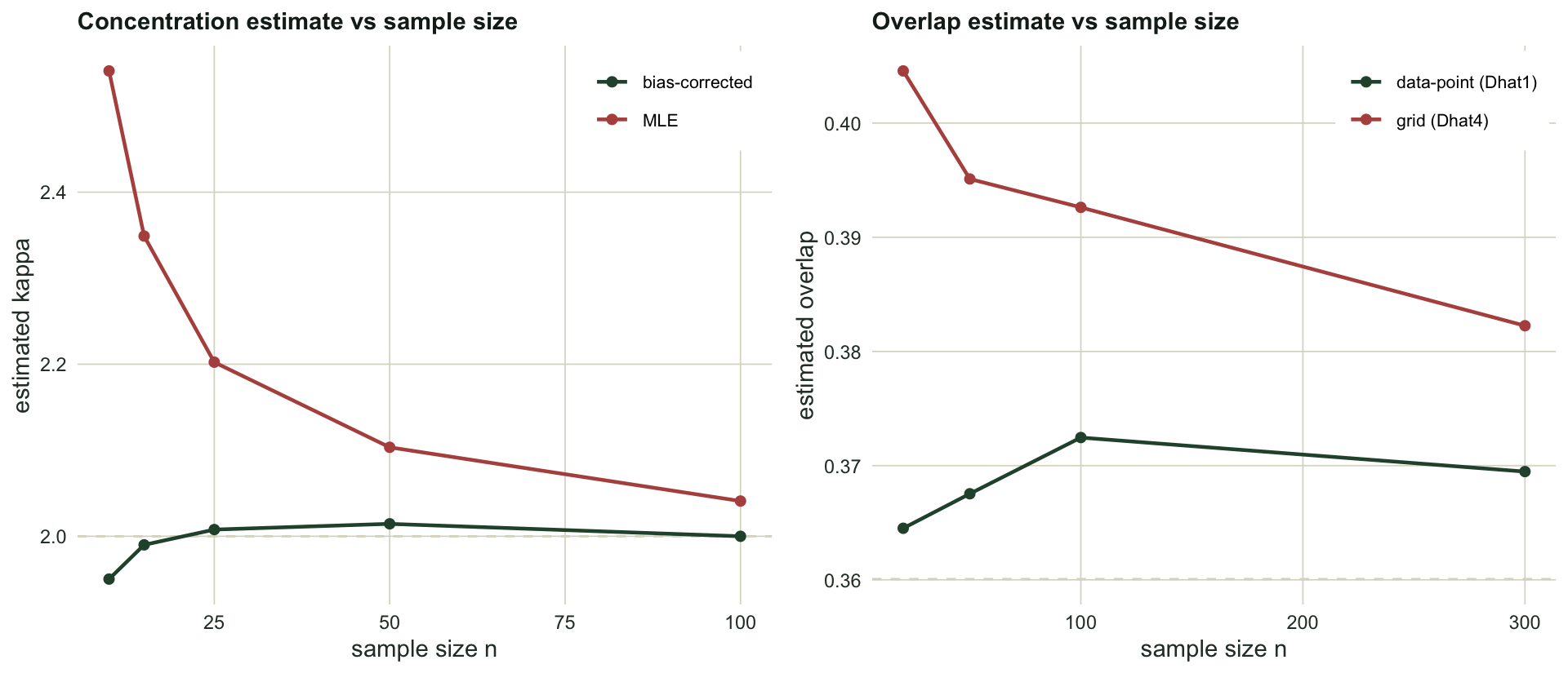
At `r kbias$n[1]` observations the maximum-likelihood estimate averages `r sprintf("%.2f", kbias$mle[1])` when the truth is `r sprintf("%.0f", kappa_true)`, an overestimate of around `r sprintf("%.0f", (kbias$mle[1] / kappa_true - 1) * 100)` per cent, so the animals look more tightly oriented than they are. The bias fades as the sample grows, reaching `r sprintf("%.2f", kbias$mle[nrow(kbias)])` by `r kbias$n[nrow(kbias)]` observations. The bias correction of Best and Fisher (1981), applied in the second column, removes almost all of it at every sample size. The check is simple: with fewer than a few dozen angles, report the bias-corrected concentration, not the raw maximum-likelihood value.
## The overlap coefficient is smoothed and biased
The overlap coefficient carries both a bias and a bandwidth dependence, and only a simulation against a known truth exposes them. Build two activity densities whose true overlap can be computed exactly, then estimate it from finite samples with the recommended bandwidth that tightens as the sample grows.
```{r}
#| label: overlap-bias
hour2rad <- function(h) 2 * pi * h / 24
fa <- function(t) dvm(t, hour2rad(0), 2)
fb <- function(t) 0.5 * dvm(t, hour2rad(6), 4) + 0.5 * dvm(t, hour2rad(18), 4)
gT <- seq(0, 2 * pi, length.out = 20001)[-20001]
D_true <- sum(pmin(fa(gT), fb(gT))) * (2 * pi / 20000)

oD4 <- function(A, B, kbw, ng = 256) { g <- seq(0, 2 * pi, length.out = ng + 1)[-(ng + 1)]
  sum(pmin(ckde(g, A, kbw), ckde(g, B, kbw))) * (2 * pi / ng) }
oD1 <- function(A, B, kbw) 0.5 * (mean(pmin(1, ckde(A, B, kbw) / ckde(A, A, kbw))) +
                                  mean(pmin(1, ckde(B, A, kbw) / ckde(B, B, kbw))))
kbw_adaptive <- function(n) 3.17 * n^0.4                 # tightens as n grows

obias <- do.call(rbind, lapply(c(20, 50, 100, 300), function(n) {
  set.seed(900 + n)
  res <- t(replicate(800, { A <- rvm(n, hour2rad(0), 2); B <- rmix(n, hour2rad(c(6, 18)), c(4, 4), c(0.5, 0.5))
    kb <- kbw_adaptive(n); c(oD4(A, B, kb), oD1(A, B, kb)) }))
  data.frame(n = n, Dhat4 = mean(res[, 1]), Dhat1 = mean(res[, 2]), SD4 = sd(res[, 1]))
}))
round(cbind(obias, true = D_true), 3)
```
The true overlap is `r sprintf("%.2f", D_true)`. The grid estimator overshoots it at every sample size, by about `r sprintf("%.2f", obias$Dhat4[1] - D_true)` at `r obias$n[1]` detections, shrinking towards `r sprintf("%.2f", obias$Dhat4[nrow(obias)] - D_true)` at `r obias$n[nrow(obias)]`. The upward bias is the smoothing showing through: kernel densities are wider than the truth, and wider curves share more area. The data-point estimator carries far less bias in this simulation. The labels in the code and figure are the reverse of those in Ridout and Linkie and the overlap package, where Dhat1 is the grid estimator, the one they recommend for small samples, and Dhat4 is the data-point estimator, recommended for larger ones. On top of the bias sits the variability, a standard deviation of about `r sprintf("%.2f", obias$SD4[1])` at the smallest sample, which is what made the bootstrap interval in the previous post so wide.
```{r}
#| label: fig-bias
#| echo: false
#| fig-cap: "Left: the mean maximum-likelihood concentration (points) overshoots the true value of two (dashed) at small samples, while the bias-corrected estimate tracks it. Right: the grid overlap estimator sits above the true overlap (dashed) and converges slowly, whereas the data-point estimator stays close to the truth."
#| fig-alt: "Left panel plots two curves of estimated concentration against sample size: the maximum-likelihood curve starts near 2.5 and falls towards 2, the corrected curve starts just below the dashed line at 2 and settles on it. Right panel plots two overlap curves against sample size: the grid estimator sits above the dashed true value and declines slowly, the data-point estimator sits close to the dashed line."
#| fig-width: 10
#| fig-height: 4.3
kl <- rbind(data.frame(n = kbias$n, val = kbias$mle, est = "MLE"),
data.frame(n = kbias$n, val = kbias$corrected, est = "bias-corrected"))
pK <- ggplot(kl, aes(n, val, colour = est)) +
geom_hline(yintercept = kappa_true, linetype = "dashed", colour = te_line) +
geom_line(linewidth = 0.8) + geom_point(size = 1.8) +
scale_colour_manual(values = c(MLE = te_rust, `bias-corrected` = te_forest)) +
labs(title = "Concentration estimate vs sample size", x = "sample size n", y = "estimated kappa") +
theme_te(11) + theme(legend.position = "inside", legend.position.inside = c(0.99, 0.99), legend.justification = c(1, 1),
legend.title = element_blank(), legend.text = element_text(size = 8),
legend.background = element_rect(fill = "white", colour = NA))
ol <- rbind(data.frame(n = obias$n, val = obias$Dhat4, est = "grid (Dhat4)"),
data.frame(n = obias$n, val = obias$Dhat1, est = "data-point (Dhat1)"))
pO <- ggplot(ol, aes(n, val, colour = est)) +
geom_hline(yintercept = D_true, linetype = "dashed", colour = te_line) +
geom_line(linewidth = 0.8) + geom_point(size = 1.8) +
scale_colour_manual(values = c(`grid (Dhat4)` = te_rust, `data-point (Dhat1)` = te_forest)) +
labs(title = "Overlap estimate vs sample size", x = "sample size n", y = "estimated overlap") +
theme_te(11) + theme(legend.position = "inside", legend.position.inside = c(0.99, 0.99), legend.justification = c(1, 1),
legend.title = element_blank(), legend.text = element_text(size = 8),
legend.background = element_rect(fill = "white", colour = NA))
grid.newpage(); pushViewport(viewport(layout = grid.layout(1, 2)))
print(pK, vp = viewport(layout.pos.row = 1, layout.pos.col = 1))
print(pO, vp = viewport(layout.pos.row = 1, layout.pos.col = 2))
```
## The through-line
None of these are exotic failures; they are the ordinary behaviour of circular summaries, and the same pattern runs through every checking post on this blog. A number that looks like a measurement, the mean direction, the concentration, the p-value, the overlap, is really the output of a choice: an assumption about how many directions the biology has, a decision about which test to run, a bandwidth, a sample size the estimator was never going to be precise at. The honest report shows the choice alongside the number. Give the resultant length with the mean direction, the test with the uniformity claim, the bandwidth and an interval with the overlap. The circle is unforgiving of summaries that pretend a distribution is simpler than it is, and the checks above are mostly ways of refusing that pretence.
## References
Batschelet E 1981 Circular Statistics in Biology. Academic Press. ISBN 978-0-12-081050-5.
Fisher NI 1993 Statistical Analysis of Circular Data. Cambridge University Press. ISBN 978-0-521-35018-1.
Mardia KV, Jupp PE 2000 Directional Statistics. Wiley. ISBN 978-0-471-95333-3.
Pewsey A, Neuhauser M, Ruxton GD 2013 Circular Statistics in R. Oxford University Press. ISBN 978-0-19-967113-7.
Best DJ, Fisher NI 1981 Communications in Statistics - Simulation and Computation 10(5):493-502 (10.1080/03610918108812225).
Watson GS 1961 Biometrika 48(1-2):109-114 (10.1093/biomet/48.1-2.109).
Ridout MS, Linkie M 2009 Journal of Agricultural, Biological, and Environmental Statistics 14(3):322-337 (10.1198/jabes.2009.08038).
Landler L, Ruxton GD, Malkemper EP 2018 Behavioral Ecology and Sociobiology 72(8):128 (10.1007/s00265-018-2538-y).
Landler L, Ruxton GD, Malkemper EP 2019 BMC Ecology 19:30 (10.1186/s12898-019-0246-8).
## Related tutorials
- [Circular data and the von Mises distribution](../circular-data-and-von-mises/)
- [Testing for circular uniformity](../testing-for-circular-uniformity/)
- [Comparing two groups of angles](../comparing-two-groups-of-angles/)
- [Activity patterns and temporal overlap](../activity-patterns-and-temporal-overlap/)