circ_R <- function(th) sqrt(mean(cos(th))^2 + mean(sin(th))^2)

# Rayleigh: based on the resultant length; large R is evidence of a single direction
rayleigh_Z <- function(th) length(th) * circ_R(th)^2

# Rao's spacing: based on how evenly the gaps between sorted angles are spread
rao_U <- function(th) {
  n <- length(th); a <- sort(th %% (2 * pi))
  gaps <- c(diff(a), 2 * pi - (a[n] - a[1]))          # arcs between neighbours, wrap included
  0.5 * sum(abs(gaps - 2 * pi / n))
}

# Kuiper: a rotation-invariant Kolmogorov-Smirnov statistic on the circle
kuiper_V <- function(th) {
  n <- length(th); u <- sort((th %% (2 * pi)) / (2 * pi))
  max((1:n) / n - u) + max(u - (0:(n - 1)) / n)
}

# Watson U-squared: a rotation-invariant Cramer-von Mises statistic
watson_U2 <- function(th) {
  n <- length(th); u <- sort((th %% (2 * pi)) / (2 * pi)); ubar <- mean(u); i <- 1:n
  sum((u - (2 * i - 1) / (2 * n))^2) + 1 / (12 * n) - n * (ubar - 0.5)^2
}

allstats <- function(th) c(Rayleigh = rayleigh_Z(th), Rao = rao_U(th),
Kuiper = kuiper_V(th), Watson = watson_U2(th))Testing for circular uniformity
R
circular statistics
hypothesis testing
ecology tutorial
ggplot2
Is there a preferred direction at all? The Rayleigh, Rao spacing, Kuiper and Watson tests in base R, and why the popular Rayleigh test misses two-way patterns.
Corrected 27 September 2026: the power section said Rao’s spacing test lags a little behind the other tests against a single preferred direction; at 0.70 against about 1.00 it lags well behind, and the text now says so.
Before summarising a set of angles with a mean direction, there is a prior question: is there a preferred direction at all, or are the angles scattered evenly around the circle? Uniformity is the natural null hypothesis for orientation, activity timing and dispersal bearings, and several tests exist for it. They are not interchangeable. The test most ecologists reach for, the Rayleigh test, cannot see one of the most biologically common departures from uniformity, and swapping it for the wrong alternative can turn a real pattern into a non-result.
This post builds four uniformity tests by hand in base R, checks that they hold their size, and then compares their power against two kinds of structure: a single preferred direction and a two-way axis.
Four tests, one null
Uniformity on the circle can fail in different ways, and each test is tuned to notice different failures.
The Rayleigh test starts from the mean resultant length of the previous post: a large R means the unit vectors add up to a long arrow, which is evidence of a single preferred direction. That is its strength and, as we will see, its weakness. The other three are omnibus tests. Rao’s spacing looks at whether the gaps between neighbouring angles are more uneven than chance would give, as they are when the angles clump. Kuiper and Watson compare the empirical distribution of angles against the flat uniform distribution, both built to be rotation-invariant so the answer does not depend on where you place the zero.
Rather than juggle a different table of critical values for each test, calibrate all four from the same simulated null: draw many uniform samples of the same size, compute every statistic, and read off the distribution under the null directly.
Setup: packages, colours and plot theme
library(ggplot2)
library(grid)
te_forest <- "#275139"; te_paper <- "#f5f4ee"; te_ink <- "#16241d"
te_body <- "#2c3a31"; te_line <- "#dad9ca"; te_sage <- "#93a87f"; te_label <- "#46604a"
te_amber <- "#cda23f"; te_rust <- "#b5534e"; te_slate <- "#5d6b61"
theme_te <- function(base_size = 11) {
  theme_minimal(base_size = base_size) +
    theme(plot.title = element_text(colour = te_ink, face = "bold", size = rel(1.0)),
          plot.subtitle = element_text(colour = te_label, size = rel(0.85)),
          axis.title = element_text(colour = te_body), axis.text = element_text(colour = te_body),
          panel.grid.major = element_line(colour = te_line, linewidth = 0.3),
          panel.grid.minor = element_blank(),
          plot.background = element_rect(fill = "#f5f4ee", colour = NA),
          panel.background = element_rect(fill = "#f5f4ee", colour = NA), legend.position = "none")
}
comp_x <- function(b) sin(b); comp_y <- function(b) cos(b)
compass_base <- function() {
  ang <- seq(0, 2 * pi, length.out = 200); circ <- data.frame(x = cos(ang), y = sin(ang))
  ticks <- seq(0, 3 * pi / 2, by = pi / 2)
  tk <- data.frame(x0 = 0.98 * sin(ticks), y0 = 0.98 * cos(ticks),
                   x1 = 1.06 * sin(ticks), y1 = 1.06 * cos(ticks))
  lab <- data.frame(x = 1.20 * sin(ticks), y = 1.20 * cos(ticks), lab = c("N", "E", "S", "W"))
  list(geom_path(data = circ, aes(x, y), colour = te_line, linewidth = 0.5),
       geom_segment(data = tk, aes(x = x0, y = y0, xend = x1, yend = y1), colour = te_sage, linewidth = 0.5),
       geom_text(data = lab, aes(x, y, label = lab), colour = te_label, size = 3.0),
       coord_fixed(xlim = c(-1.32, 1.32), ylim = c(-1.32, 1.32)), theme_void(),
       theme(plot.title = element_text(colour = te_ink, face = "bold", size = 11, hjust = 0.5),
             plot.background = element_rect(fill = "#f5f4ee", colour = NA)))
}
rvm <- function(n, mu, kappa) {
  out <- numeric(n); a <- 1 + sqrt(1 + 4 * kappa^2); b <- (a - sqrt(2 * a)) / (2 * kappa)
  r <- (1 + b^2) / (2 * b); i <- 0
  while (i < n) { u1 <- runif(1); z <- cos(pi * u1); f <- (1 + r * z) / (r + z); c1 <- kappa * (r - f); u2 <- runif(1)
    if (c1 * (2 - c1) - u2 > 0 || log(c1 / u2) + 1 - c1 >= 0) {
      u3 <- runif(1); i <- i + 1; out[i] <- (mu + sign(u3 - 0.5) * acos(f)) %% (2 * pi) } }
  out
}
# a two-way axis: half the angles pointing one way, half the opposite way
raxial <- function(n, mu, kappa) { s <- rvm(n, mu, kappa); fl <- runif(n) < 0.5; s[fl] <- (s[fl] + pi) %% (2 * pi); s }
mc_null <- function(n, B, seed) { set.seed(seed); t(replicate(B, allstats(runif(n, 0, 2 * pi)))) }
n <- 60
null_dist <- mc_null(n, B = 5000, seed = 808) # 5000 uniform samples of size 60
pvalue <- function(obs) sapply(seq_len(4), function(j) mean(null_dist[, j] >= obs[j]))Two datasets, two verdicts
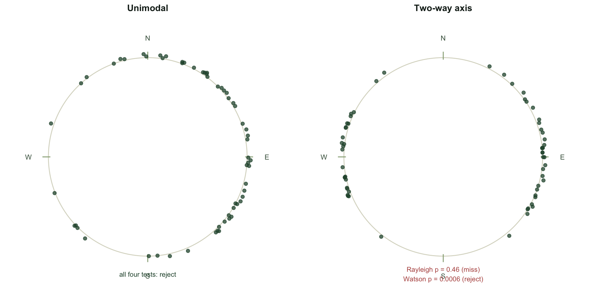
Take two synthetic samples of 60 angles. The first has a single preferred direction (a von Mises with moderate concentration). The second is a two-way axis: the same shape, but half the angles are flipped to point the opposite way, as animals moving up and down a valley or along a fence line would produce.
set.seed(4251)
unimodal <- rvm(n, mu = pi / 2, kappa = 1.2)
set.seed(4300)
axial    <- raxial(n, mu = pi / 2, kappa = 4)

p_uni <- pvalue(allstats(unimodal))
p_axi <- pvalue(allstats(axial))
round(rbind(unimodal = p_uni, axial = p_axi), 4)
[,1] [,2] [,3] [,4]
unimodal 0.0000 0.0044 0 0e+00
axial 0.4602 0.0000 0 6e-04For the unimodal sample the mean resultant length is 0.44, and every test rejects uniformity: the Rayleigh p-value is below 0.001, and Rao, Kuiper and Watson agree.
The axial sample is where the tests part company. Its mean resultant length is only 0.115, because the two opposite clusters cancel almost perfectly. The Rayleigh test reads that near-zero resultant and concludes there is no preferred direction, returning a p-value of 0.46. That is the wrong conclusion: the angles are strongly patterned, just not around a single direction. Watson (p = 0.0006), Kuiper and Rao all reject uniformity, because they respond to the shape of the whole distribution, not only to a single resultant.
Which test sees what
One sample proves nothing on its own, so measure the tests properly by simulation. Fix the size at five per cent using the same null, then estimate power against a unimodal alternative and against a two-way axis across a range of concentrations.
crit <- apply(null_dist, 2, quantile, 0.95)               # 5% critical values from the shared null

power_for <- function(gen, B, seed) {
  set.seed(seed); S <- t(replicate(B, allstats(gen())))
  colMeans(sweep(S, 2, crit, ">="))
}
B <- 4000
size    <- power_for(function() runif(n, 0, 2 * pi), B, 5001)   # should sit near 0.05
pow_uni <- power_for(function() rvm(n, pi / 2, 1.0), B, 5002)   # single direction
pow_ax2 <- power_for(function() raxial(n, pi / 2, 2), B, 5003)  # weak two-way axis
pow_ax4 <- power_for(function() raxial(n, pi / 2, 4), B, 5004)  # strong two-way axis
round(rbind(size = size, unimodal = pow_uni, axis_k2 = pow_ax2, axis_k4 = pow_ax4), 3)
Rayleigh Rao Kuiper Watson
size 0.046 0.042 0.049 0.047
unimodal 0.998 0.697 0.995 0.998
axis_k2 0.059 0.284 0.334 0.254
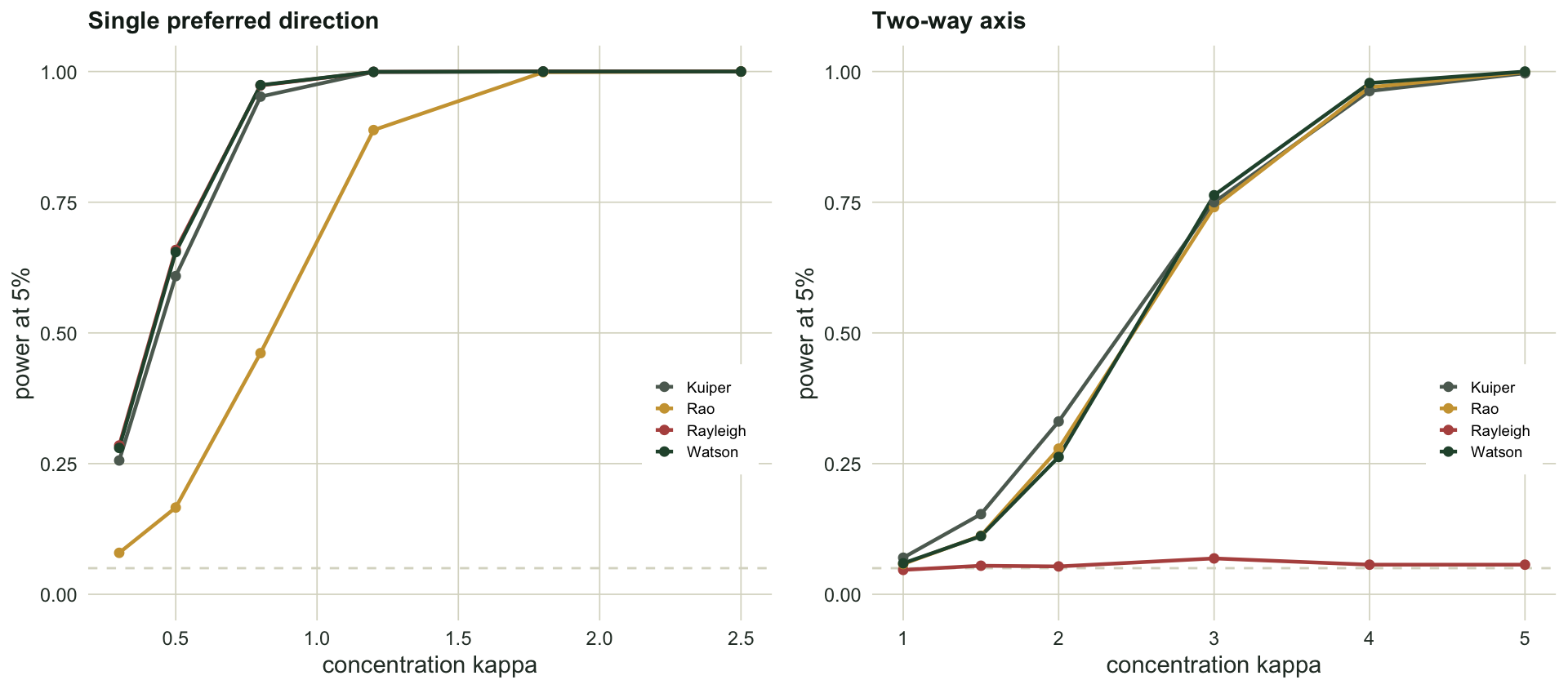
axis_k4 0.066 0.968 0.960 0.982Every test holds its size near five per cent, so the comparison is fair. Against a single preferred direction the Rayleigh test is as good as any, with power 1.00, and Kuiper and Watson match it; Rao’s spacing lags well behind at 0.70, because it is not tuned for smooth single peaks.
The axial alternative reverses the picture. The Rayleigh test never gets off the floor: its power is 0.059 against a weak axis and still only 0.066 against a strong one, barely above its five per cent false-positive rate. It is not underpowered here, it is blind: a two-way axis produces a near-zero resultant no matter how tight the clusters are, so the statistic the test is built on carries no signal. The omnibus tests climb as the clusters tighten, from between a quarter and a third at the weak axis to 0.98 for Watson at the strong one.
Choosing a test
The moral is not that the Rayleigh test is bad. Against the alternative it was built for, a single concentrated direction, it is the most powerful of the four, and that is often exactly the ecological question: do the animals head somewhere in particular. The mistake is using it as a general test of uniformity when the biology might produce two-way or multi-way structure. Bimodal orientation is common: bidirectional movement along corridors, escape headings away from a threat, bimodal activity with dawn and dusk peaks once time is wrapped onto the circle. For those, an omnibus test is essential, and recent work in ecology recommends exactly this shift away from a reflexive Rayleigh test (Landler, Ruxton and Malkemper 2018, 2019).
The deeper point runs through this series. A test answers the question its statistic encodes, no more. The Rayleigh test asks “is the resultant long”, which is not the same as “is the distribution non-uniform”, and the gap between those two questions is where a real pattern can vanish. The checking post at the end returns to how the choice of test, and the modality you assume, decide what a circular analysis is allowed to conclude.
References
Batschelet E 1981 Circular Statistics in Biology. Academic Press. ISBN 978-0-12-081050-5.
Fisher NI 1993 Statistical Analysis of Circular Data. Cambridge University Press. ISBN 978-0-521-35018-1.
Mardia KV, Jupp PE 2000 Directional Statistics. Wiley. ISBN 978-0-471-95333-3.
Pewsey A, Neuhauser M, Ruxton GD 2013 Circular Statistics in R. Oxford University Press. ISBN 978-0-19-967113-7.
Rayleigh 1919 Philosophical Magazine Series 6 37(220):321-347 (10.1080/14786440408635894).
Kuiper NH 1960 Proceedings of the Koninklijke Nederlandse Akademie van Wetenschappen Series A 63:38-47 (10.1016/S1385-7258(60)50006-0).
Watson GS 1961 Biometrika 48(1-2):109-114 (10.1093/biomet/48.1-2.109).
Rao JS 1976 Sankhya Series B 38(4):329-338.
Landler L, Ruxton GD, Malkemper EP 2018 Behavioral Ecology and Sociobiology 72(8):128 (10.1007/s00265-018-2538-y).
Landler L, Ruxton GD, Malkemper EP 2019 BMC Ecology 19:30 (10.1186/s12898-019-0246-8).