---
title: "Circular data and the von Mises distribution"
description: "Why arithmetic means fail on the circle: the mean direction and resultant length for animal orientations, and fitting a von Mises distribution in base R."
date: "2026-06-08 10:00"
categories: [R, circular statistics, directional data, ecology tutorial, ggplot2]
image: thumbnail.png
image-alt: "A single stylised circular diagram headed von Mises, with the subtitle mean direction plus concentration. A rose of twelve sectors of unequal length sits inside a tilted dark green ring, all of it within a thin outer circle, and one arrow runs from the centre up and to the right at about 45 degrees, along the longest sector."
---
Ecologists collect angles more often than they realise. Compass bearings of departing birds, the aspect of a nest slope, the time of day an animal is active, the flowering date on the annual cycle: all of these live on a circle, not on a line. The awkward part is that the number 359 and the number 1 are two degrees apart, not 358, and every ordinary summary you reach for assumes the opposite. This post sets out the base-R toolkit for angular data: the mean direction, the mean resultant length as a measure of concentration, and the von Mises distribution, the circular counterpart of the normal.
Everything here is hand-coded with base `stats` plus `ggplot2`. There is no circular-statistics package to install, and building the pieces yourself makes the assumptions visible.
## The wrap-around trap
Take five bearings clustered around north: 350, 10, 20, 340 and 0 degrees. By eye they point north. The arithmetic mean does not.
```{r}
#| label: setup
#| message: false
#| warning: false
#| code-fold: true
#| code-summary: "Setup: packages, colours and plot theme"
library(ggplot2)
library(grid)

te_forest <- "#275139"; te_paper <- "#f5f4ee"; te_ink <- "#16241d"
te_body <- "#2c3a31"; te_line <- "#dad9ca"; te_sage <- "#93a87f"; te_label <- "#46604a"
te_amber <- "#cda23f"; te_rust <- "#b5534e"
theme_te <- function(base_size = 11) {
  theme_minimal(base_size = base_size) +
    theme(plot.title = element_text(colour = te_ink, face = "bold", size = rel(1.0)),
          plot.subtitle = element_text(colour = te_label, size = rel(0.85)),
          axis.title = element_text(colour = te_body),
          axis.text = element_text(colour = te_body),
          panel.grid.major = element_line(colour = te_line, linewidth = 0.3),
          panel.grid.minor = element_blank(),
          plot.background = element_rect(fill = "#f5f4ee", colour = NA),
          panel.background = element_rect(fill = "#f5f4ee", colour = NA),
          legend.position = "none")
}
comp_x <- function(b) sin(b); comp_y <- function(b) cos(b)
compass_base <- function() {
  ang <- seq(0, 2 * pi, length.out = 200)
  circ <- data.frame(x = cos(ang), y = sin(ang))
  ticks <- seq(0, 3 * pi / 2, by = pi / 2)
  tk <- data.frame(x0 = 0.98 * sin(ticks), y0 = 0.98 * cos(ticks),
                   x1 = 1.06 * sin(ticks), y1 = 1.06 * cos(ticks))
  lab <- data.frame(x = 1.20 * sin(ticks), y = 1.20 * cos(ticks), lab = c("N", "E", "S", "W"))
  list(geom_path(data = circ, aes(x, y), colour = te_line, linewidth = 0.5),
       geom_segment(data = tk, aes(x = x0, y = y0, xend = x1, yend = y1), colour = te_sage, linewidth = 0.5),
       geom_text(data = lab, aes(x, y, label = lab), colour = te_label, size = 3.2),
       coord_fixed(xlim = c(-1.32, 1.32), ylim = c(-1.32, 1.32)), theme_void(),
       theme(plot.title = element_text(colour = te_ink, face = "bold", size = 11, hjust = 0.5),
             plot.background = element_rect(fill = "#f5f4ee", colour = NA)))
}
# von Mises rejection sampler (Best and Fisher 1979), base R only
rvm <- function(n, mu, kappa) {
  out <- numeric(n); a <- 1 + sqrt(1 + 4 * kappa^2); b <- (a - sqrt(2 * a)) / (2 * kappa)
  r <- (1 + b^2) / (2 * b); i <- 0
  while (i < n) {
    u1 <- runif(1); z <- cos(pi * u1); f <- (1 + r * z) / (r + z); c1 <- kappa * (r - f); u2 <- runif(1)
    if (c1 * (2 - c1) - u2 > 0 || log(c1 / u2) + 1 - c1 >= 0) {
      u3 <- runif(1); i <- i + 1; out[i] <- (mu + sign(u3 - 0.5) * acos(f)) %% (2 * pi)
    }
  }
  out
}
```
```{r}
#| label: trap
# work in radians throughout; degrees only for display
deg2rad <- function(d) d * pi / 180
rad2deg <- function(r) r * 180 / pi

circ_mean <- function(theta) atan2(mean(sin(theta)), mean(cos(theta)))   # in (-pi, pi]

bearings  <- c(350, 10, 20, 340, 0)
arith     <- mean(bearings)                                              # naive linear mean
circular  <- rad2deg(circ_mean(deg2rad(bearings)))                       # correct mean direction, (-180, 180]
circular  <- ifelse(abs(circular) < 0.5, 0, circular %% 360)            # tidy the exact-north case
c(arithmetic = arith, circular = circular)
```
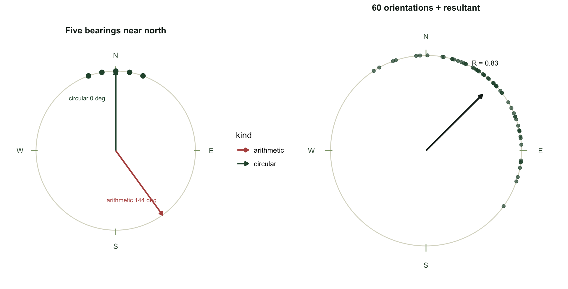
The arithmetic mean returns `r sprintf("%.0f", mean(c(350, 10, 20, 340, 0)))` degrees, pointing south-east, because it cannot see that 350 and 10 are neighbours. The circular mean returns `r sprintf("%.0f", circular)` degrees, which is north. The fix is to average the unit vectors, not the raw numbers: replace each angle by its point on the unit circle, sum the horizontal and vertical components, and take the direction of the total. That single idea drives everything below.
## Mean direction and resultant length
For a sample of angles the two building blocks are the mean cosine and mean sine. Their vector length is the *mean resultant length*, written R, and its direction is the *mean direction*.
```{r}
#| label: summaries
circ_R <- function(theta) sqrt(mean(cos(theta))^2 + mean(sin(theta))^2)  # resultant length in [0, 1]

# synthetic orientations: 60 departure bearings, illustrative only
set.seed(4250)
theta <- rvm(60, mu = deg2rad(40), kappa = 3.0)

Rbar     <- circ_R(theta)
mean_dir <- rad2deg(circ_mean(theta)) %% 360
circ_var <- 1 - Rbar                       # circular variance in [0, 1]
circ_sd  <- rad2deg(sqrt(-2 * log(Rbar)))  # circular standard deviation, degrees
round(c(Rbar = Rbar, mean_dir = mean_dir, circ_var = circ_var, circ_sd = circ_sd), 3)
```
The resultant length is `r sprintf("%.3f", Rbar)`, a number between zero and one. At one, every angle is identical; at zero, the angles cancel out and there is no preferred direction. This is a moderately tight cluster, with a mean direction of `r sprintf("%.1f", mean_dir)` degrees and a circular standard deviation of `r sprintf("%.1f", circ_sd)` degrees.
The trap from the first section is not a toy. The arithmetic mean of these same 60 bearings is `r sprintf("%.1f", mean(rad2deg(theta)))` degrees, off by more than thirty degrees, because a handful of angles fall just below 360 and drag the linear average upward. The circular mean is immune to where you place the zero.
```{r}
#| label: fig-compass
#| fig-cap: "Left: five bearings near north, with the arithmetic mean (rust) pointing the wrong way and the circular mean (green) pointing north. Right: 60 synthetic orientations with the mean resultant vector; its length R measures concentration."
#| fig-alt: "Two compass plots. The left shows five points near the top of the circle with a green arrow pointing up and a rust arrow pointing down-right. The right shows sixty points clustered top-right with a single arrow of length 0.83 pointing towards forty-five degrees."
#| fig-width: 10
#| fig-height: 5.1
#| code-fold: true
#| code-summary: "Show the code behind this output"
mean_toy  <- circ_mean(deg2rad(bearings)) %% (2 * pi)
arith_toy <- deg2rad(mean(bearings))
ptsA <- data.frame(x = comp_x(deg2rad(bearings)), y = comp_y(deg2rad(bearings)))
arrA <- data.frame(x0 = 0, y0 = 0,
                   x1 = c(comp_x(mean_toy), comp_x(arith_toy)),
                   y1 = c(comp_y(mean_toy), comp_y(arith_toy)),
                   kind = c("circular", "arithmetic"))
pA <- ggplot() + compass_base() +
  geom_point(data = ptsA, aes(x, y), colour = te_forest, size = 2.6) +
  geom_segment(data = arrA, aes(x = x0, y = y0, xend = x1, yend = y1, colour = kind),
               arrow = arrow(length = unit(0.16, "cm"), type = "closed"), linewidth = 0.9) +
  scale_colour_manual(values = c(circular = te_forest, arithmetic = te_rust)) +
  annotate("text", x = -0.36, y = 0.66, label = "circular 0 deg", colour = te_forest, size = 2.7) +
  annotate("text", x = 0.36, y = -0.62, label = "arithmetic 144 deg", colour = te_rust, size = 2.7,
           hjust = 1) +
  ggtitle("Five bearings near north")

mdir_r <- circ_mean(theta) %% (2 * pi)
ptsB <- data.frame(x = comp_x(theta), y = comp_y(theta))
arrB <- data.frame(x0 = 0, y0 = 0, x1 = Rbar * comp_x(mdir_r), y1 = Rbar * comp_y(mdir_r))
pB <- ggplot() + compass_base() +
  geom_point(data = ptsB, aes(x, y), colour = te_forest, size = 1.7, alpha = 0.7) +
  geom_segment(data = arrB, aes(x = x0, y = y0, xend = x1, yend = y1),
               arrow = arrow(length = unit(0.16, "cm"), type = "closed"), colour = te_ink, linewidth = 1.0) +
  annotate("text", x = 0.62, y = 0.92, label = sprintf("R = %.2f", Rbar), colour = te_ink, size = 3.1) +
  ggtitle("60 orientations + resultant")

grid.newpage(); pushViewport(viewport(layout = grid.layout(1, 2)))
print(pA, vp = viewport(layout.pos.row = 1, layout.pos.col = 1))
print(pB, vp = viewport(layout.pos.row = 1, layout.pos.col = 2))
```
## The von Mises distribution
The normal distribution does not wrap, so it cannot describe angles. Its circular replacement is the von Mises distribution, with a mean direction `mu` and a concentration `kappa`. The density is
```
f(theta) = exp(kappa * cos(theta - mu)) / (2 * pi * I0(kappa))
```
where `I0` is the modified Bessel function of the first kind, order zero, available in base R as `besselI(kappa, 0)`. When `kappa` is zero the distribution is uniform on the circle; as `kappa` grows it concentrates around `mu`, and for large `kappa` it looks almost normal.
Maximum likelihood is unusually clean. The estimate of `mu` is simply the mean direction, and the estimate of `kappa` solves `A(kappa) = R`, where `A` is the ratio of two Bessel functions. There is no closed form, so solve it numerically.
```{r}
#| label: vonmises-fit
dvm     <- function(x, mu, kappa) exp(kappa * cos(x - mu)) / (2 * pi * besselI(kappa, 0))
A_kappa <- function(kappa) besselI(kappa, 1) / besselI(kappa, 0)

kappa_mle <- function(Rbar) {
  if (Rbar < 1e-8)      return(0)
  if (Rbar > 0.999999)  return(Inf)
  uniroot(function(k) A_kappa(k) - Rbar, interval = c(1e-6, 700))$root
}

kappa_hat <- kappa_mle(Rbar)
kappa_hat
```
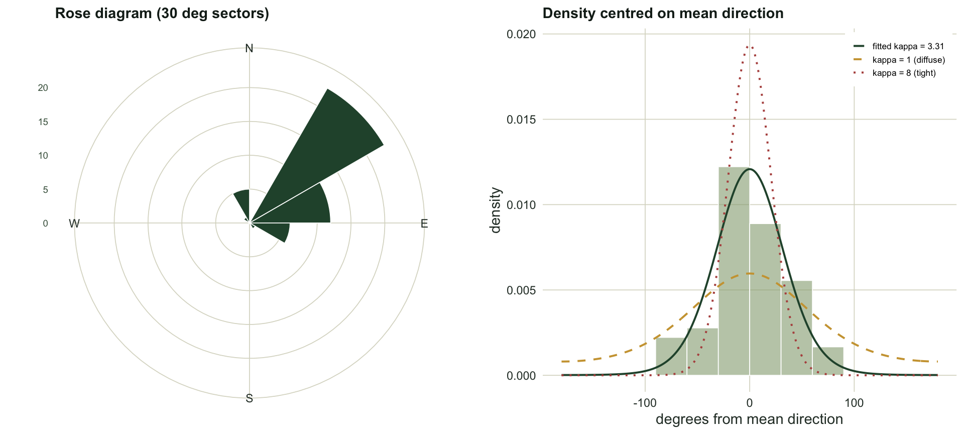
The fitted concentration is `r sprintf("%.2f", kappa_hat)`. That is the value that makes the theoretical resultant length `A(kappa)` match the observed `r sprintf("%.2f", Rbar)`.
One caution worth carrying forward: the maximum-likelihood `kappa` is biased upward in small samples, sometimes badly. The standard correction (Best and Fisher 1981) nudges it back:
```{r}
#| label: kappa-bias
kappa_bc <- function(k, n) {
  if (!is.finite(k)) return(k)
  if (k < 2) return(max(k - 2 / (n * k), 0))
  (n - 1)^3 * k / (n^3 + n)
}
kappa_star <- kappa_bc(kappa_hat, length(theta))
kappa_star
```
The corrected value is `r sprintf("%.2f", kappa_star)`, a little lower. With sixty angles the difference is small; with fifteen it would not be, and the checking post in this series returns to how far the reported concentration can drift from the truth.
```{r}
#| label: fig-vonmises
#| fig-cap: "Left: a rose diagram of the 60 orientations in 30-degree sectors. Right: the same data unrolled and centred on the mean direction, with the fitted von Mises density and two reference concentrations. Larger kappa means a tighter peak."
#| fig-alt: "Left panel is a rose diagram with the longest wedges near north-east. Right panel is a histogram with three density curves: the fitted kappa of 3.3 in green tracks the histogram, a diffuse kappa of 1 in amber is nearly flat, and a tight kappa of 8 in rust is a narrow spike."
#| fig-width: 10
#| fig-height: 4.5
#| code-fold: true
#| code-summary: "Code behind this output; later chunks use it, so run it first"
brks <- seq(0, 2 * pi, length.out = 13); mids <- (head(brks, -1) + tail(brks, -1)) / 2
cnt  <- as.integer(table(cut(theta, brks, include.lowest = TRUE)))
rose <- data.frame(mid_deg = rad2deg(mids), count = cnt)
pRose <- ggplot(rose, aes(x = mid_deg, y = count)) +
  geom_col(width = 30, fill = te_forest, colour = "white", linewidth = 0.3) +
  coord_polar(start = 0, direction = 1) +
  # rad2deg(pi/12) is 14.999999999999998, so the first sector's lower edge sits a
  # floating-point hair below 0; the default oob rule would censor that whole wedge
  scale_x_continuous(limits = c(0, 360), breaks = c(0, 90, 180, 270),
                     labels = c("N", "E", "S", "W"), oob = scales::oob_keep) +
  labs(title = "Rose diagram (30 deg sectors)", x = NULL, y = NULL) +
  theme_te(11) + theme(axis.text.y = element_text(size = 7, colour = te_label))

rel <- ((theta - mdir_r + pi) %% (2 * pi)) - pi
dfh <- data.frame(rel_deg = rad2deg(rel))
xs  <- seq(-pi, pi, length.out = 400)
lab_fit <- sprintf("fitted kappa = %.2f", kappa_hat)
curveDf <- rbind(
  data.frame(x = rad2deg(xs), dens = dvm(xs, 0, kappa_hat), k = lab_fit),
  data.frame(x = rad2deg(xs), dens = dvm(xs, 0, 1), k = "kappa = 1 (diffuse)"),
  data.frame(x = rad2deg(xs), dens = dvm(xs, 0, 8), k = "kappa = 8 (tight)"))
pB2 <- ggplot() +
  geom_histogram(data = dfh, aes(x = rel_deg, y = after_stat(density)),
                 binwidth = 30, boundary = 0, fill = te_sage, colour = "white", alpha = 0.6, linewidth = 0.3) +
  geom_line(data = curveDf, aes(x = x, y = dens * pi / 180, linetype = k, colour = k), linewidth = 0.7) +
  scale_colour_manual(values = setNames(c(te_forest, te_amber, te_rust),
                       c(lab_fit, "kappa = 1 (diffuse)", "kappa = 8 (tight)"))) +
  scale_linetype_manual(values = setNames(c("solid", "dashed", "dotted"),
                       c(lab_fit, "kappa = 1 (diffuse)", "kappa = 8 (tight)"))) +
  labs(title = "Density centred on mean direction", x = "degrees from mean direction", y = "density") +
  theme_te(11) + theme(legend.position = "inside", legend.position.inside = c(0.99, 0.99), legend.justification = c(1, 1),
                       legend.title = element_blank(), legend.text = element_text(size = 6.5),
                       legend.key.size = unit(0.35, "cm"),
                       legend.background = element_rect(fill = "white", colour = NA))

grid.newpage(); pushViewport(viewport(layout = grid.layout(1, 2)))
print(pRose, vp = viewport(layout.pos.row = 1, layout.pos.col = 1))
print(pB2, vp = viewport(layout.pos.row = 1, layout.pos.col = 2))
```
## Grouped data
Field bearings often arrive already binned into sectors, and the same summaries work from counts. Weight each sector midpoint by its count, average the components, and read off the resultant.
```{r}
#| label: grouped
Cg <- sum(cnt * cos(mids)) / sum(cnt)
Sg <- sum(cnt * sin(mids)) / sum(cnt)
Rbar_g <- sqrt(Cg^2 + Sg^2)
mean_dir_g <- rad2deg(atan2(Sg, Cg)) %% 360
round(c(Rbar_grouped = Rbar_g, mean_dir_grouped = mean_dir_g), 3)
```
The grouped resultant length is `r sprintf("%.2f", Rbar_g)` against `r sprintf("%.2f", Rbar)` for the raw angles, and the grouped mean direction is `r sprintf("%.1f", mean_dir_g)` degrees against `r sprintf("%.1f", mean_dir)`. Binning into twelve sectors costs almost nothing here, though very coarse sectors would smear a tight cluster.
## What R does not tell you
The mean direction and resultant length describe the data as though a single preferred direction exists. That assumption is doing quiet work. If animals move along a two-way axis, say up and down a valley, the angles split into two opposite clusters, the components cancel, and R collapses towards zero even though the pattern is strongly structured. A near-zero R can mean "no preferred direction" or "two opposite directions", and the mean direction becomes meaningless. Reporting R alone would hide the difference.
That is the reason the next post in this series asks a sharper question before any of these summaries: is there a preferred direction at all, and which test can actually see the structure that is present. The checking post at the end returns to how modality, sample size and the choice of test decide what a circular summary is allowed to claim.
## References
Batschelet E 1981 Circular Statistics in Biology. Academic Press. ISBN 978-0-12-081050-5.
Fisher NI 1993 Statistical Analysis of Circular Data. Cambridge University Press. ISBN 978-0-521-35018-1.
Mardia KV, Jupp PE 2000 Directional Statistics. Wiley. ISBN 978-0-471-95333-3.
Jammalamadaka SR, SenGupta A 2001 Topics in Circular Statistics. World Scientific. ISBN 978-981-02-3778-3.
Pewsey A, Neuhauser M, Ruxton GD 2013 Circular Statistics in R. Oxford University Press. ISBN 978-0-19-967113-7.
Best DJ, Fisher NI 1979 Applied Statistics 28(2):152-157 (10.2307/2346732).
Best DJ, Fisher NI 1981 Communications in Statistics - Simulation and Computation 10(5):493-502 (10.1080/03610918108812225).
## Related tutorials
- [Testing for circular uniformity](../testing-for-circular-uniformity/)
- [Comparing two groups of angles](../comparing-two-groups-of-angles/)
- [Checking a circular analysis](../checking-a-circular-analysis/)
- [Phenology in R: day of year and event timing](../phenology-and-day-of-year/)