inside <- function(P, r, half) {
  (P[, 1]^2 + P[, 2]^2 <= r^2) & (abs(atan2(P[, 2], P[, 1])) <= half)
}

crossings <- function(P1, D, r, half) {
  m <- nrow(P1)
  U <- matrix(Inf, m, 4); IN <- matrix(FALSE, m, 4)
  a <- D[, 1]^2 + D[, 2]^2
  b <- 2 * (P1[, 1] * D[, 1] + P1[, 2] * D[, 2])
  cc <- P1[, 1]^2 + P1[, 2]^2 - r^2
  disc <- b^2 - 4 * a * cc
  ok <- disc > 0 & a > 0
  sq <- ifelse(ok, sqrt(pmax(disc, 0)), NA_real_)
  for (k in 1:2) {
    u <- (-b + c(-1, 1)[k] * sq) / (2 * a)
    Q <- cbind(P1[, 1] + u * D[, 1], P1[, 2] + u * D[, 2])
    good <- ok & !is.na(u) & u > 0 & u <= 1 & abs(atan2(Q[, 2], Q[, 1])) <= half
    good[is.na(good)] <- FALSE
    U[good, k] <- u[good]
    IN[good, k] <- ((D[, 1] * Q[, 1] + D[, 2] * Q[, 2]) < 0)[good]
  }
  for (k in 1:2) {
    s <- c(1, -1)[k] * half
    e <- c(cos(s), sin(s))
    nrm <- c(cos(s + c(1, -1)[k] * pi / 2), sin(s + c(1, -1)[k] * pi / 2))
    cD <- D[, 1] * e[2] - D[, 2] * e[1]
    u <- -(P1[, 1] * e[2] - P1[, 2] * e[1]) / cD
    tt <- (P1[, 1] + u * D[, 1]) * e[1] + (P1[, 2] + u * D[, 2]) * e[2]
    good <- abs(cD) > 1e-12 & !is.na(u) & u > 0 & u <= 1 & tt >= 0 & tt <= r
    good[is.na(good)] <- FALSE
    U[good, 2 + k] <- u[good]
    IN[good, 2 + k] <- ((D[, 1] * nrm[1] + D[, 2] * nrm[2]) < 0)[good]
  }
  list(U = U, IN = IN)
}

## returns the times of every entry into the zone, per animal
entry_times <- function(nstep, dt, v, W, r, half, rho) {
  u <- runif(nstep)
  turn <- 2 * atan(((1 - rho) / (1 + rho)) * tan(pi * (u - 0.5)))
  phi <- runif(1, 0, 2 * pi) + cumsum(turn)
  D <- cbind(v * dt * cos(phi), v * dt * sin(phi))
  p0 <- c(runif(1, -W / 2, W / 2), runif(1, -W / 2, W / 2))
  X <- p0[1] + cumsum(D[, 1]); Y <- p0[2] + cumsum(D[, 2])
  P1 <- cbind(c(p0[1], X[-nstep]), c(p0[2], Y[-nstep]))
  R1 <- cbind(((P1[, 1] + W / 2) %% W) - W / 2, ((P1[, 2] + W / 2) %% W) - W / 2)
  idx <- which((R1[, 1]^2 + R1[, 2]^2) < (r + v * dt)^2)
  if (!length(idx)) return(numeric(0))
  cr <- crossings(R1[idx, , drop = FALSE], D[idx, , drop = FALSE], r, half)
  hit <- which(is.finite(cr$U), arr.ind = TRUE)
  if (!nrow(hit)) return(numeric(0))
  tt <- (idx[hit[, 1]] - 1 + cr$U[hit]) * dt
  sort(tt[cr$IN[hit]])
}

rem_D <- function(y, t, v, r, theta) y * pi / (t * v * r * (2 + theta))Checking a camera trap density estimate
R
camera traps
abundance
ecology tutorial
Three checks for a random encounter model density estimate in R: the independence filter, interval coverage in a patchy landscape, and where the error lives.
Corrected 14 October 2026: the post called its filter table a lower bound on the size of the mistake, which holds only on these simulated records, and now says that the long-window losses come from how often an animal returns to the camera on this small torus, so they are smaller where animals return less often; and its finding that clumped crossings leave the Poisson interval intact is now limited to the persistent walker it was shown for, since a more tortuous animal gives a much larger standard error.
Corrected 1 October 2026: the post now says that its independence filter runs over each animal’s own records, the most lenient form of the species rule, so the filter table is a lower bound on the loss; and the claim that precision is bought with locations rather than nights is now limited to this survey, where a typical camera records hundreds of crossings.
You have a density. It came out of a formula with four inputs, three of which you measured badly and one of which you counted. This post is about finding out how much of it to believe, and it is arranged around the checks that pay: what the independence filter does to the estimate, whether the interval covers, and which input the uncertainty actually comes from. The last section is about the one that no check catches.
The setup is the gas from the encounter rate post, with the same exact crossing geometry.
Check 1: what the independence filter costs
Camera trap protocols almost always collapse detections that arrive close together. The usual rule is that records of the same species within some window, thirty minutes being the folk standard, count as one independent event. The reason given is that consecutive photographs of the same animal are not independent, which is true and which is beside the point here.
The gas model does not want independent events. It wants boundary crossings, because that is what the flux formula counts. Every time an animal re-enters the detection zone it has crossed the boundary again and the theory has already accounted for it. Filter those out and you are estimating the rate of something the formula does not describe.
Here is a survey with the filter applied at a range of windows. It runs over each animal’s own records, the most lenient version of the rule: a camera that cannot tell unmarked animals apart has to run it over the whole species, which never discards fewer.
W <- 20; r <- 4; half <- 20 * pi / 180; v <- 1; dt <- 0.5
A <- W^2; nanim <- 120; nstep <- 20000; Tt <- nstep * dt; Dtrue <- nanim / A

set.seed(3301)
ev <- lapply(seq_len(nanim), function(i) entry_times(nstep, dt, v, W, r, half, rho = 0.9))

## a filter with window w keeps an entry only if the previous kept entry, for the
## same animal, was more than w seconds ago
apply_filter <- function(ev, w) {
  sum(vapply(ev, function(x) {
    if (!length(x)) return(0L)
    keep <- 1L; last <- x[1]
    for (s in x[-1]) if (s - last > w) { keep <- keep + 1L; last <- s }
    keep
  }, integer(1)))
}

wins <- c(0, 1, 5, 30, 300, 1800)
flt <- data.frame(window_s = wins)
flt$y <- vapply(wins, function(w) apply_filter(ev, w), numeric(1))
flt$D_hat <- rem_D(flt$y, Tt, v, r, 2 * half)
flt$ratio_to_truth <- flt$D_hat / Dtrue
flt
window_s y D_hat ratio_to_truth
1 0 10440 0.30389758 1.01299192
2 1 10370 0.30185995 1.00619983
3 5 9547 0.27790327 0.92634424
4 30 8062 0.23467646 0.78225487
5 300 2895 0.08427045 0.28090149
6 1800 699 0.02034717 0.06782388The unfiltered count is the right one: it recovers 1.01 times the truth. A one second window costs only 1 per cent, but by five seconds 9 per cent of the crossings are gone, because a wandering animal crosses the zone edge repeatedly on its way through. The thirty minute standard returns 0.07 times the truth: at that point you are counting animal-visits to the neighbourhood, not boundary crossings, and the formula has no idea.
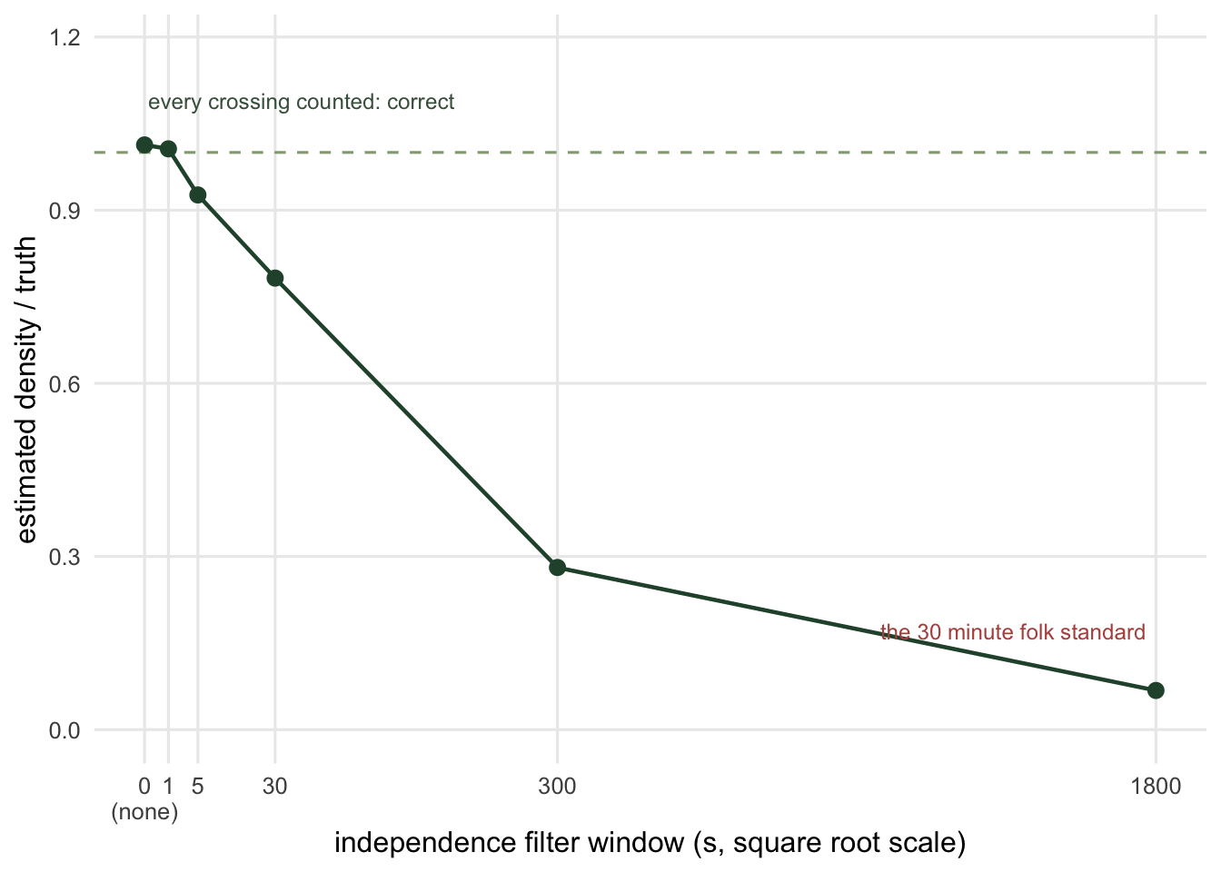
The practical trouble is that a real camera does not report boundary crossings. It reports triggers, with a recovery time between them, and a burst of five photographs of one deer is genuinely one crossing seen five times. So you do need a filter, set to something like the sensor’s own recovery time, to convert triggers into crossings. What you must not do is set it to thirty minutes because a paper about occupancy said so. The two filters have the same name and opposite jobs. On these records the table is a lower bound on the size of the mistake, since a filter run over the whole species never discards fewer. Its long-window rows, though, belong to this small torus: each animal enters the zone about once every 115 seconds on average, so a thirty minute window can keep at most 6 of the 87 or so entries an animal makes in the run, and at a camera that animals revisit less often the long windows cost less.
Check 2: does the interval cover?
The encounter count is the one thing you truly measure, so the temptation is to treat \(y\) as Poisson and put \(\sqrt{y}\) around it. The encounter rate post gave a reason to distrust that: a wandering animal delivers its crossings in clumps, and a sum over clusters is not a sum over events. Run many independent cameras over identical gas and see how much damage that does.
set.seed(3302)
ncam <- 400; nsm <- 4000; nan_c <- 20
Tc <- nsm * dt; Dbar <- nan_c / A

one_count <- function(n) sum(vapply(seq_len(n), function(i)
  length(entry_times(nsm, dt, v, W, r, half, rho = 0.9)), integer(1)))

y_hom <- vapply(seq_len(ncam), function(k) one_count(nan_c), numeric(1))
c(mean_count = mean(y_hom), var_count = var(y_hom),
  variance_to_mean = var(y_hom) / mean(y_hom))
mean_count var_count variance_to_mean
342.560000 383.284612 1.118883 Barely any: the variance is 1.12 times the mean. The clustering is real but it is small, because a persistent walker crosses the zone and leaves rather than loitering on the boundary. So for an animal this persistent the thing that is supposed to break the Poisson interval does not, and if the landscape were as uniform as this torus you could use \(\sqrt{y}\) and sleep soundly. The warning still stands for a more tortuous animal, whose standard error the encounter rate post found several times larger.
Landscapes are not uniform. Give each camera its own local density, drawn with a coefficient of variation of 0.5, which is a modest amount of patchiness for a real species, and leave everything else alone.
set.seed(3303)
cv_local <- 0.5
D_local <- rlnorm(ncam, log(Dbar) - log(1 + cv_local^2) / 2, sqrt(log(1 + cv_local^2)))
y_het <- vapply(D_local, function(d) one_count(max(1, round(d * A))), numeric(1))

c(mean_count = mean(y_het), var_count = var(y_het),
  variance_to_mean = var(y_het) / mean(y_het))
mean_count var_count variance_to_mean
338.5925 26143.9112 77.2135 The variance to mean ratio is now 77. Nothing about the counting changed: the extra spread is the landscape, arriving through the front door. Now ask how often each interval catches the truth, in surveys of ten cameras.
per_survey <- 10
grp <- function(y) split(y, rep(seq_len(length(y) / per_survey), each = per_survey))

pois_ci <- function(y) {                       # pooled count treated as Poisson
  s <- sum(y); t_tot <- per_survey * Tc
  rem_D(s + c(-1, 1) * 1.96 * sqrt(s), t_tot, v, r, 2 * half)
}
camera_ci <- function(y) {                     # cameras as the replicate unit
  d <- rem_D(y, Tc, v, r, 2 * half)
  mean(d) + c(-1, 1) * qt(0.975, length(d) - 1) * sd(d) / sqrt(length(d))
}
cover <- function(y, ci) mean(vapply(grp(y), function(g) {
  b <- ci(g); Dbar >= b[1] && Dbar <= b[2]
}, logical(1)))

data.frame(
  landscape = c("uniform", "uniform", "patchy (CV 0.5)", "patchy (CV 0.5)"),
  interval = rep(c("Poisson on the pooled count", "t interval across cameras"), 2),
  coverage = c(cover(y_hom, pois_ci), cover(y_hom, camera_ci),
               cover(y_het, pois_ci), cover(y_het, camera_ci)),
  nominal = 0.95)
landscape interval coverage nominal
1 uniform Poisson on the pooled count 0.950 0.95
2 uniform t interval across cameras 0.975 0.95
3 patchy (CV 0.5) Poisson on the pooled count 0.250 0.95
4 patchy (CV 0.5) t interval across cameras 0.925 0.95On the uniform torus both intervals are fine. On the patchy one the Poisson interval collapses to 25 per cent coverage while the camera-level interval holds. The lesson is not that Poisson is wrong in principle, it is that, for an animal this persistent, Poisson is an assumption about the landscape rather than about the counter, and you cannot check it from the pooled count. Treat the cameras as the replicate unit and you never have to: the spread across cameras absorbs the patchiness, the counting noise and anything else that varies between locations, at the cost of a wider and honest interval.
Check 3: where the uncertainty comes from
Now assume the count is handled. The estimate is \(\hat{D} = y\pi / (t \hat{v} r (2+\theta))\), and every symbol on the right except \(t\) and \(\pi\) is a measurement. Because the formula is a product of powers, the delta method is a one-liner: relative variances add.
\[\mathrm{CV}^2(\hat{D}) \approx \mathrm{CV}^2(y) + \mathrm{CV}^2(\hat{v}) + \mathrm{CV}^2(\hat{L})\]
Put in numbers a real survey would recognise. The count term is the camera-level standard error measured on the patchy landscape above, for a survey of ten cameras. The speed comes from a few hundred camera passages with a harmonic mean correction, which Rowcliffe et al. (2016) put at a coefficient of variation of roughly 0.15 to 0.25 for a decent sample. The detection zone comes from an adapted distance sampling fit (Rowcliffe et al. 2011), which is not free either.
cv_count <- sd(rem_D(y_het, Tc, v, r, 2 * half)) /
  (mean(rem_D(y_het, Tc, v, r, 2 * half)) * sqrt(per_survey))   # 10 cameras, patchy
cvs <- c(count = cv_count, speed = 0.20, zone = 0.10)
tot <- sqrt(sum(cvs^2))
rbind(component_CV = round(c(cvs, total = tot), 4),
      share_of_variance = round(c(cvs^2 / tot^2, total = 1), 4))
count speed zone total
component_CV 0.1510 0.2000 0.1000 0.2698
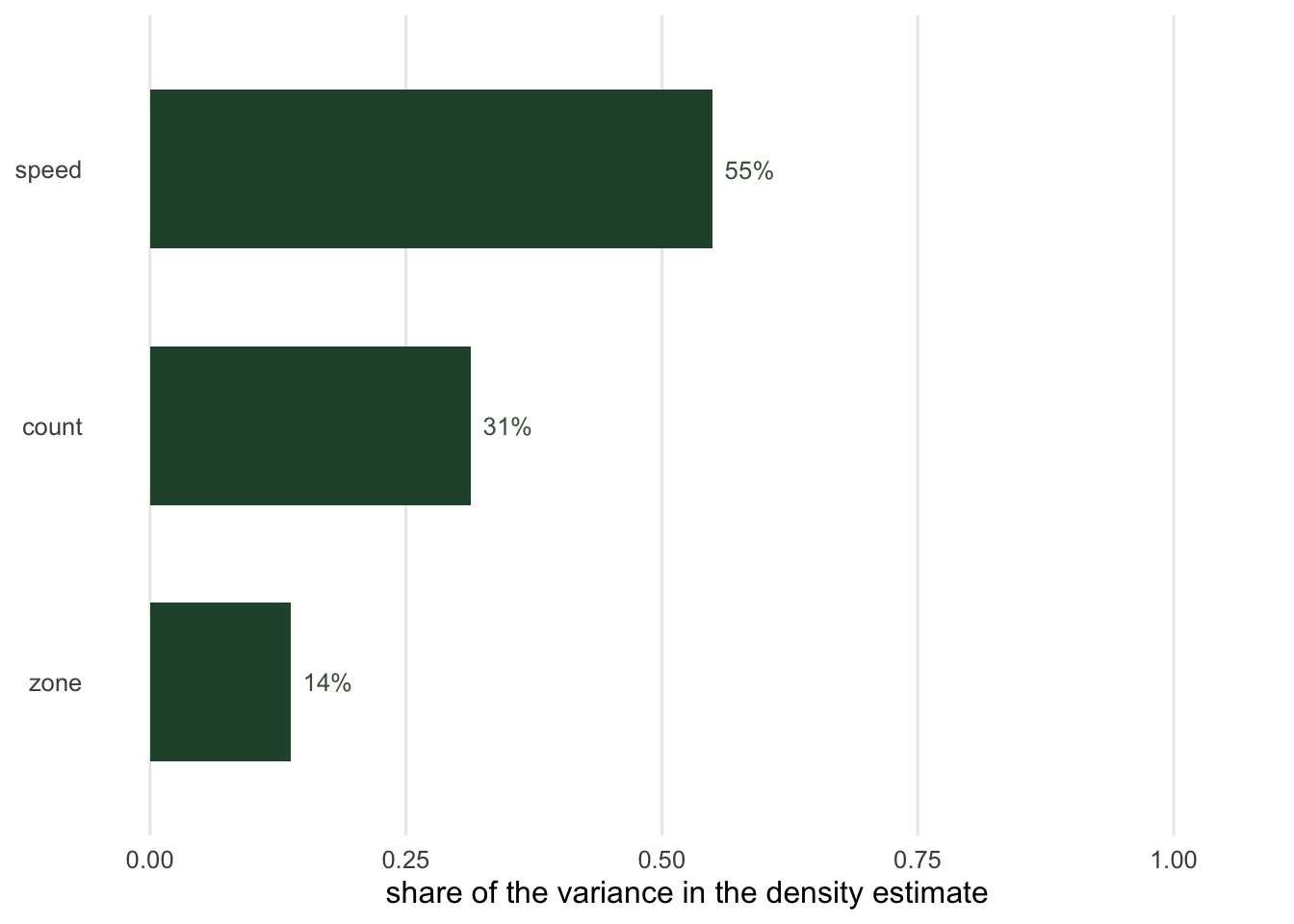
share_of_variance 0.3132 0.5494 0.1374 1.0000The speed contributes 55 per cent of the variance, the count 31 per cent and the zone the rest. Two things follow, and the second is the practical message of the whole cluster.
The count term is not counting noise. It is the spread between cameras, divided by the square root of ten. Running each camera for twice as long barely moves it, because a camera in a poor patch stays in a poor patch; running twice as many cameras does move it. In this survey, where a typical camera records hundreds of crossings, effort and precision are related through the number of locations, not the number of nights, which is the opposite of the intuition that a camera trap survey is a counting exercise.
And a perfect count would not help much. Set the count term to zero and the coefficient of variation on the density only falls from 0.27 to 0.22, because the speed and the zone were measured rather than counted and they do not care how many cameras you own. The route to a tighter density estimate runs through a better speed: more passages measured well, an external day range from telemetry, or the staying time model, which trades the speed measurement for a staying time measurement and its own set of problems.
The honest limit: the cameras are where you put them
Every check above is internal. Here is the one that is not, and it cannot be made internal.
The flux argument is local. An encounter rate at a camera is set by the density of animals at that camera, so a random encounter model estimate is an estimate of the local density, faithfully and precisely. Whether that number means anything about the landscape depends entirely on how the camera got there.
Take a landscape with two habitats of equal area, one good and one poor, and a field team that does what field teams do: put the cameras where the animals are.
set.seed(3304)
one_camera <- function(D_hab) {                       # a camera in its own habitat
  rem_D(one_count(round(D_hab * A)), Tc, v, r, 2 * half)
}
D_good <- 0.50; D_poor <- 0.10
truth_landscape <- (D_good + D_poor) / 2               # habitats are equal in area

good <- vapply(seq_len(8), function(i) one_camera(D_good), numeric(1))
poor <- vapply(seq_len(2), function(i) one_camera(D_poor), numeric(1))

data.frame(
  quantity = c("cameras in good habitat", "cameras in poor habitat",
               "unweighted mean of the 10 cameras", "area-weighted mean",
               "true landscape density"),
  value = c(mean(good), mean(poor), mean(c(good, poor)),
            (mean(good) + mean(poor)) / 2, truth_landscape))
quantity value
1 cameras in good habitat 0.49652614
2 cameras in poor habitat 0.09751503
3 unweighted mean of the 10 cameras 0.41672392
4 area-weighted mean 0.29702058
5 true landscape density 0.30000000Each camera did its job: the good-habitat cameras recover 0.99 times the local density and the poor-habitat cameras 0.98 times theirs. The estimator is not broken. The survey is. Averaging the ten cameras gives 1.39 times the landscape density, because eight of the ten sit in the half where the animals are.
Now the part that matters. Go back through the three checks and run them on this survey. The counts are overdispersed, as before, and the camera-level interval is honest about the spread. The filter behaves the same way. The speed and staying-time checks from the earlier posts in this cluster have nothing to catch either: the animals move at the same speed in both habitats, and the estimate above uses that true speed. Every diagnostic in this post passes, and the answer is 39 per cent too high.
There is no residual to plot. The information that would reveal the problem, which habitat each camera sat in and how much of each habitat the landscape holds, is not in the camera data and never will be. It has to come from the sampling design: random or stratified placement, with the strata weighted by area, exactly as in design-based distance sampling. The spread across cameras is a hint that habitat matters, but a large spread is equally consistent with a well designed survey of a patchy population, so it is not a test.
So the checking list for a camera trap density estimate has an item that is not a computation. Before any of the above, write down how the camera locations were chosen. If the answer is that they went on trails, at water, or wherever the field team expected animals, the density estimate is a local density for an unspecified locality, and no amount of camera-nights, bootstrap replicates or model choice will turn it into a landscape density.
References
- Rowcliffe, Field, Turvey, Carbone 2008 Journal of Applied Ecology 45(4):1228-1236 (10.1111/j.1365-2664.2008.01473.x)
- Rowcliffe, Carbone, Jansen, Kays, Kranstauber 2011 Methods in Ecology and Evolution 2(5):464-476 (10.1111/j.2041-210X.2011.00094.x)
- Rowcliffe, Jansen, Kays, Kranstauber, Carbone 2016 Remote Sensing in Ecology and Conservation 2(2):84-94 (10.1002/rse2.17)
- Palencia, Rowcliffe, Vicente, Acevedo 2021 Journal of Applied Ecology 58:1583-1592 (10.1111/1365-2664.13913)
- Hutchinson, Waser 2007 Biological Reviews 82(3):335-359 (10.1111/j.1469-185X.2007.00014.x)