library(ggplot2)
te_canvas <- theme(plot.background  = element_rect(fill = "#f5f4ee", colour = NA),
                   panel.background = element_rect(fill = "#f5f4ee", colour = NA))

g_hn  <- function(x, s) exp(-x^2/(2*s^2))
mu_hn <- function(s, w) sqrt(2*pi)*s*(pnorm(w, 0, s) - 0.5)
ld_hn <- function(x, s, w) -x^2/(2*s^2) - log(mu_hn(s, w))
g_hr  <- function(x, s, b) 1 - exp(-(x/s)^(-b))
mu_hr <- function(s, b, w) integrate(g_hr, 0, w, s = s, b = b)$value
fit_hn <- function(x, w) exp(optimise(function(p) -sum(ld_hn(x, exp(p), w)),
                                      c(-8, 1), tol = 1e-10)$minimum)
w <- 0.1Checking a distance sampling model
R
distance sampling
model checking
abundance
ecology tutorial
The goodness-of-fit test accepts surveys whose density is 12 per cent wrong, and the assumption that matters most leaves no trace in the likelihood at all.
Corrected 7 October 2026: the double observer section said that where the heterogeneity lives decides the answer and how much of it there is does not; the two worlds were matched on the amount, which also changes how much of the gap an estimator closes when its independence assumption fails, and the text now says so; the first section also said that a spike at zero distance, a hole in the histogram and heaping on round numbers all show up in the goodness-of-fit test, and it now says that only gross problems that change the counts in its five bins do, while animals near the line recorded at zero, a modest spike or heaping on finer round numbers often pass.
Corrected 1 October 2026: the closing section said that what kept the pooled estimate from unbiasedness was the amount of heterogeneity rather than the shape of the key; it now says the shortfall comes from the key, because a key that followed the pooled shape exactly would be unbiased.
Updated 27 September 2026: a new section, When the tail is left in, measures what fitting out to the largest recorded distance does to density when detections have a long tail, at three tail lengths, against cutting the farthest 10 per cent, and the checklist gains a row for it.
Three posts in this series have shown a distance sampling analysis returning a confident wrong number: a pooled detection function reversing which habitat is denser, a half-normal at a point inflating density by a sixth, a hierarchical model halving a population when the animals hold still.
The reasonable response is to ask what you would check. Distance sampling has a natural answer, because unlike most ecological models it makes a direct, testable prediction about data you can see: the histogram of distances should look like the fitted curve. So plot it, run a goodness-of-fit test, and if it passes, you are fine.
This post takes that programme seriously and measures how much protection it buys. The honest answer is: some, and a good deal less than the ritual implies.
The check that works
Start with the good news, because there is some. Bin the distances, fit the key function, compare observed counts against expected counts with a chi-square statistic. Before trusting a test to reject a bad model, check that it accepts a good one at the advertised rate: a test with the wrong size is not evidence, it is a coin with an opinion.
cut <- seq(0, w, length.out = 6)
pi_hn <- function(s) { P <- sqrt(2*pi)*s*(pnorm(cut[-1], 0, s) - pnorm(cut[-6], 0, s))/w
                       P/sum(P) }
gof_hn <- function(x) {
  s  <- fit_hn(x, w)
  ob <- tabulate(findInterval(x, cut, rightmost.closed = TRUE), 5)
  ex <- length(x)*pi_hn(s)
  c(p = pchisq(sum((ob - ex)^2/ex), df = 5 - 1 - 1, lower.tail = FALSE), sigma = s)
}
## a world where the half-normal is exactly right
s_ok <- 0.045; D0 <- 100; L_ok <- 266/(2*D0*mu_hn(s_ok, w))
cal <- t(sapply(1:400, function(i) {
  set.seed(61000 + i)
  N <- rpois(1, D0*2*w*L_ok); x <- runif(N, 0, w)
  gof_hn(x[runif(N) < g_hn(x, s_ok)])
}))
sprintf("model-true data, n approx 266: test rejects at 0.05 in %.1f%% of surveys | median p %.3f",
        100*mean(cal[, "p"] < 0.05), median(cal[, "p"]))
[1] "model-true data, n approx 266: test rejects at 0.05 in 6.0% of surveys | median p 0.493"Well behaved: it rejects the truth at about the nominal rate, so it is a real test rather than a formality. It can also catch gross problems that change the relative counts in its five bins, such as a deep hole in the histogram or heavy heaping on coarse round numbers. Others often pass: animals near the line recorded at zero stay in the first bin and leave its counts unchanged, and a modest spike at zero or heaping on finer round numbers changes the counts too little to be caught reliably. Those are for the histogram itself, drawn at finer bins.
What it misses
Now give it the job it is actually asked to do. The true detection function has a shoulder, generated by a hazard-rate key. You fit a half-normal, which cannot make a shoulder. From the point transect post, we know this costs about 11 per cent on a line. Does the test tell you?
s_hr <- 0.05; b_hr <- 3
mu_t <- mu_hr(s_hr, b_hr, w); Ln <- 266/(2*D0*mu_t)
res <- t(sapply(1:400, function(i) {
  set.seed(63000 + i)
  N <- rpois(1, D0*2*w*Ln); x <- runif(N, 0, w)
  x <- x[runif(N) < g_hr(x, s_hr, b_hr)]
  g <- gof_hn(x)
  c(p = g["p"], bias = length(x)/(2*Ln*mu_hn(g["sigma"], w))/D0 - 1, n = length(x))
}))
acc <- res[res[, 1] > 0.05, ]
sprintf("half-normal fitted to hazard-rate data (n approx %.0f, 5 bins, df 3):", mean(res[, 3]))
[1] "half-normal fitted to hazard-rate data (n approx 268, 5 bins, df 3):"sprintf(" rejects at 0.05: %.1f%% of surveys | median p-value %.3f | mean density bias %+.1f%%",
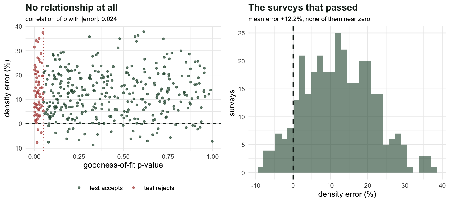
100*mean(res[, 1] < 0.05), median(res[, 1]), 100*mean(res[, 2]))[1] " rejects at 0.05: 17.2% of surveys | median p-value 0.312 | mean density bias +12.4%"sprintf(" among the surveys the test ACCEPTS: mean bias %+.1f%%, worst %+.1f%%",
100*mean(acc[, 2]), 100*max(acc[, 2]))[1] " among the surveys the test ACCEPTS: mean bias +12.2%, worst +37.8%"sprintf(" correlation between the p-value and |bias|: %.3f", cor(res[, 1], abs(res[, 2])))[1] " correlation between the p-value and |bias|: 0.024"Read those three lines slowly.
The test rejects the wrong model in 17 per cent of surveys, so 83 per cent of the time it hands the wrong model a clean bill of health. That is a power problem, and power problems are familiar and forgivable.
The second line is the one that should worry you. Among the surveys that pass, the mean density bias is +12.2 per cent, which is the same as the mean bias across all surveys. Passing the test tells you nothing about whether your density is right. The worst passing survey is out by 38 per cent, and it passed.
And the third line says it exactly: the correlation between the p-value and the size of the error is 0.024. Not weak. Zero, to within the noise of 400 surveys. The statistic the test computes and the quantity you care about are unrelated.
A goodness-of-fit test asks whether the fitted curve describes the shape of the histogram. Your density estimate depends on the height of that curve at zero. Those are different questions, and a model can answer the first one well while getting the second one wrong, because five bins of a smooth curve leave plenty of room to be wrong in the corner where nobody is looking.
The assumption with no fingerprints
That was the diagnostic being weak. This one is different in kind.
Every density estimate in this series divides by an effective width computed on the assumption that \(g(0) = 1\): everything on the transect line is detected. It is the first assumption in every textbook, and it is the one that fails most often in practice. Divers miss animals below them. Aerial observers miss animals under the plane. A bird singing directly overhead in the canopy is not obviously easier to detect than one at 20 m.
Suppose it is false, and the true detection function is \(c \cdot g(x)\) for some \(c < 1\). Fit your model to the distances and see what happens.
set.seed(4283)
s_t <- 0.05; L <- 30; Dtrue <- 60
N <- rpois(1, Dtrue*2*w*L); xa <- runif(N, 0, w)
x <- xa[runif(N) < g_hn(xa, s_t)]
base <- optimise(function(p) -sum(ld_hn(x, exp(p), w)), c(-8, 1), tol = 1e-12)
out <- t(sapply(c(1, 0.8, 0.6, 0.4), function(g0) {
  ## the world where only a fraction g0 of the animals on the line are seen
  nll <- function(p) { s <- exp(p)
    -sum(log(g0*g_hn(x, s)) - log(g0*mu_hn(s, w))) }
  o <- optimise(nll, c(-8, 1), tol = 1e-12)
  c(g0 = g0, sigma = exp(o$minimum), d_sigma = exp(o$minimum) - exp(base$minimum),
    loglik = -o$objective, d_loglik = -o$objective + base$objective,
    D = length(x)/(2*L*mu_hn(exp(o$minimum), w)*g0))
}))
sprintf("one survey, n = %d detections", length(x))
[1] "one survey, n = 223 detections"print(round(out, 8)) g0 sigma d_sigma loglik d_loglik D
[1,] 1.0 0.05705162 0 531.7441 0 56.47631
[2,] 0.8 0.05705162 0 531.7441 0 70.59539
[3,] 0.6 0.05705162 0 531.7441 0 94.12719
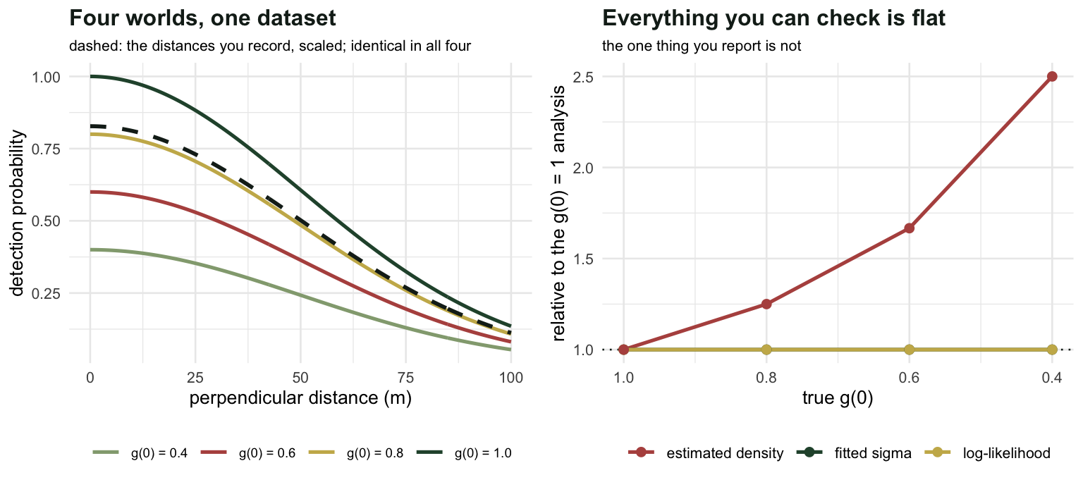
[4,] 0.4 0.05705162 0 531.7441 0 141.19078Look at the middle columns. The fitted scale is the same in all four rows, and so is the log-likelihood: those differences are not small, they are zero to the last bit an optimiser can carry. Meanwhile the density runs from 56.5 to 141.2, a factor of 2.5.
This is not a weak diagnostic. It is an exact invariance, and it takes one line of algebra to see why. The likelihood is built from the probability density of the observed distances,
\[f(x) = \frac{c\,g(x)}{\int_0^w c\,g(t)\,\mathrm{d}t} = \frac{g(x)}{\mu}\]
and the constant cancels. Your distances are conditional on detection, so they know the shape of the detection function and nothing whatsoever about its height. Every estimate in the series assumes \(g(0) = 1\), so when \(g(0) = c\) it is too low by the factor \(c\), and the true density is \(\hat{D}/c\): +25 per cent relative to the estimate at \(c = 0.8\), +67 per cent at \(c = 0.6\), +150 per cent at \(c = 0.4\).
No goodness-of-fit test can see this, because the fit is identical. No residual can see it. No AIC comparison can see it, because both models have the same likelihood and the same parameter count. There is no diagnostic, no plot and no statistic in R that will tell you, because the information is not in the data. The assumption you most need is the one your survey cannot check.
When the tail is left in
Every survey so far was generated only out to 100 m, so none of these fits has met a tail. Recorded distances often end in a long, thin one, a few animals seen far beyond the rest, and the textbook step is to cut the farthest 5 to 10 per cent of distances before fitting (Buckland et al. 2015). For a model without covariates, the defaults of ds() in the Distance package (read in its source, version 2.0.1.9000) do not cut: the truncation distance is the largest observed distance, the key is a half-normal, cosine adjustments of order 2, 3 and upwards are added one at a time for as long as AIC improves, up to max_adjustments = 5, and the curve is held strictly non-increasing. Cutting is one argument: ds(distances, truncation = "10%"). This post does not run ds(). The fitter below follows the same recipe, so its numbers describe the recipe and not the package, whose own optimiser decides where its selection stops: a half-normal key, cosine terms of order 2 to 6, the curve held non-increasing at 20 equally spaced points (the number the ds() help gives; the mrds code that ds() calls uses 10), and forward selection that stops at the first model with a worse AIC.
## g = key x (1 + cosines); centred cosines give, for fixed sigma, a concave log-likelihood
tr_fitk <- function(x, tw, k) {                    # k cosine terms, orders 2 to k + 1
  cosm <- function(z) outer(z, seq_len(k) + 1, function(z, j) cos(j*pi*z/tw))
  xq <- (1:1000 - 0.5)*tw/1000; xm <- seq(0, tw, length.out = 20)  # quadrature, monotonicity
  Cq <- cosm(xq); Cx <- cosm(x); Cm <- cosm(xm)
  prof <- function(s) {                            # sigma fixed: best coefficients
    kq <- g_hn(xq, s); m0 <- mean(kq)*tw; ll0 <- -sum(x^2)/(2*s^2) - length(x)*log(m0)
    if (k == 0) return(list(ll = ll0, f0 = 1/m0, ok = TRUE))
    cbar <- colMeans(kq*Cq)*tw/m0; E <- sweep(Cx, 2, cbar); M <- sweep(Cm, 2, cbar)
    r <- exp(-diff(xm^2)/(2*s^2))                  # constraints: g falls, g(tw) >= 0
    A <- rbind(M[-20, , drop = FALSE] - r*M[-1, , drop = FALSE], M[20, ]); b <- c(r - 1, -1)
    cf <- rep(0, k); u <- rep(1, length(x)); ok <- FALSE
    for (it in 1:80) {                             # Newton steps under the constraints
      Eu <- E/u
      grad <- colSums(Eu)
      H <- crossprod(Eu) + diag(1e-10*max(1, Eu^2), k)
      move <- tryCatch(quadprog::solve.QP(H, grad, t(A), pmin(b - drop(A %*% cf), 0))$solution,
                       error = function(e) NULL)
      ok <- !is.null(move) && sum(grad*move) < 1e-9   # converged
      if (is.null(move) || ok) break
      a <- 1
      repeat {                                     # halve the step until the fit improves
        un <- 1 + drop(E %*% (cf + a*move))
        if (all(un > 0) && sum(log(un)) >= sum(log(u)) + 1e-4*a*sum(grad*move)) break
        a <- a/2
        if (a < 1e-12) break }
      ok <- a < 1e-12 && sum(grad*move) < 1e-6
      if (a < 1e-12) break                         # no step improves the fit: stop
      cf <- cf + a*move
      u <- un }
    list(ll = ll0 + sum(log(u)), f0 = (1 + sum((1 - cbar)*cf))/m0, ok = ok) }
  lg <- log(tw) + seq(log(1/200), log(20), length.out = 30)  # sigma: grid, then optimise
  pl <- sapply(lg, function(l) prof(exp(l))$ll); i <- which.max(pl)
  o <- optimise(function(l) -prof(exp(l))$ll, lg[c(max(1, i - 1), min(30, i + 1))])
  f <- prof(exp(if (-o$objective > pl[i]) o$minimum else lg[i]))
  c(f, aic = -2*f$ll + 2*(k + 1)) }
tr_ds <- function(x, tw, all_k = FALSE) {          # forward AIC: stop at the first worse model
  x <- x[x <= tw]; fits <- list(tr_fitk(x, tw, 0)); k <- NA   # k: the selected model
  for (j in 1:5) {                   # all_k = TRUE: fit every k anyway (b = 2.2 only)
    if (!is.na(k) && !all_k) break
    fits[[j + 1]] <- tr_fitk(x, tw, j)
    if (is.na(k) && (!fits[[j + 1]]$ok || fits[[j + 1]]$aic > fits[[j]]$aic)) k <- j - 1 }
  if (is.na(k)) k <- 5
  nf0 <- length(x)*sapply(fits, `[[`, "f0"); list(k = k, nf0 = nf0[k + 1], nf0_k = nf0) }
Three worlds, each with 100 animals per square kilometre, a detection scale of 0.05 km and a line length set for 266 expected detections, as before, but with animals out to 1 km, 20 times that scale: the half-normal, the hazard-rate with b = 3 from the second section, and a heavier hazard-rate tail with b = 2.2. Each of 120 surveys per world is fitted twice, at the largest distance and with the farthest 10 per cent cut. A second chunk repeats the b = 2.2 world with animals out to 0.5 km and to 2 km, 60 surveys each on the same recipe, with seeds of their own.
tr_g <- list(`half-normal` = function(x) g_hn(x, s_hr),
             `hazard-rate, b = 3` = function(x) g_hr(x, s_hr, b_hr),
             `hazard-rate, b = 2.2` = function(x) g_hr(x, s_hr, 2.2))
tr_W <- 1; tr_L <- sapply(tr_g, function(g) 266/(2*D0*integrate(g, 0, tr_W)$value))
tr_res <- do.call(rbind, lapply(1:3, function(j) t(sapply(1:120, function(i) {
  set.seed(96000 + 1000*j + i)
  N <- rpois(1, D0*2*tr_W*tr_L[j]); xa <- runif(N, 0, tr_W); x <- xa[runif(N) < tr_g[[j]](xa)]
  fm <- tr_ds(x, max(x), all_k = j == 3)           # ds() default: the largest distance
  fq <- tr_ds(x, unname(quantile(x, 0.9)))         # the farthest 10 per cent cut
  rbk <- fm$nf0_k; length(rbk) <- 6; rb <- c(fm$nf0, fq$nf0, rbk)/(2*tr_L[[j]]*D0) - 1
  c(j = j, w = max(x), k_max = fm$k, k_cut = fq$k,
    rb_max = rb[1], rb_cut = rb[2], rbk = rb[-(1:2)]) }))))
tr_cell <- function(j, h) { v <- tr_res[tr_res[, "j"] == j, ]; rb <- v[, paste0("rb_", h)]
  c(bias = mean(rb), mcse = sd(rb)/sqrt(120), median = median(rb),
    cv = sd(1 + rb)/mean(1 + rb), five_terms = mean(v[, paste0("k_", h)] == 5)) }
tr_sum <- expand.grid(w = c("max", "cut"), truth = names(tr_g), stringsAsFactors = FALSE)
tr_sum <- cbind(tr_sum, t(mapply(tr_cell, match(tr_sum$truth, names(tr_g)), tr_sum$w)))
print(tr_sum, digits = 2)
w truth bias mcse median cv five_terms
1 max half-normal -0.0021 0.0089 0.002 0.098 0.00
2 cut half-normal 0.0153 0.0105 0.013 0.113 0.00
3 max hazard-rate, b = 3 -0.0038 0.0128 0.021 0.141 0.71
4 cut hazard-rate, b = 3 0.0913 0.0094 0.082 0.095 0.00
5 max hazard-rate, b = 2.2 -0.2586 0.0084 -0.258 0.124 0.99
6 cut hazard-rate, b = 2.2 0.0846 0.0110 0.081 0.112 0.00tr_shift <- tr_res[tr_res[, "j"] == 2, "rb_cut"] - tr_res[tr_res[, "j"] == 2, "rb_max"]
tr_km <- tr_res[tr_res[, "j"] == 3, paste0("rbk", 1:6)]; tr_k <- colMeans(tr_km)
cat("b = 2.2 at the largest distance, FIXED k = 0 to 5:", sprintf("%+.3f", tr_k),
sprintf("(MC SE at most %.3f)\n", max(apply(tr_km, 2, sd))/sqrt(120)))b = 2.2 at the largest distance, FIXED k = 0 to 5: -0.530 -0.508 -0.411 -0.374 -0.319 -0.258 (MC SE at most 0.009)tr_rw <- data.frame(t(mapply(function(W, i) { # hazard-rate b = 2.2, animals out to W km
set.seed(91000 + 1000*W + i)
L <- 266/(2*D0*integrate(tr_g[[3]], 0, W)$value)
xa <- runif(rpois(1, D0*2*W*L), 0, W)
x <- xa[runif(length(xa)) < tr_g[[3]](xa)]
f <- lapply(c(max(x), unname(quantile(x, 0.9))), tr_ds, x = x) # largest distance, 10% cut
c(W = W, cap = f[[1]]$k == 5, rb = sapply(f, `[[`, "nf0")/(2*L*D0) - 1) }, # rb1, rb2
rep(c(0.5, 2), each = 60), 1:60)))
print(aggregate(. ~ W, tr_rw, function(v) c(mean = mean(v), se = sd(v)/sqrt(60))), digits = 2) W cap.mean cap.se rb1.mean rb1.se rb2.mean rb2.se
1 0.5 0.567 0.065 0.024 0.015 0.070 0.018
2 2.0 1.000 0.000 -0.494 0.014 0.067 0.014tr_step <- diff(t(tr_km)) # fixed k: paired steps, k to k + 1
cat(sprintf("steps in k: largest paired SE %.3f\n", max(apply(tr_step, 1, sd))/sqrt(120)))steps in k: largest paired SE 0.003With the heavy tail the largest distance averages 0.83 km, forward selection runs to the five-term cap in 99 per cent of fits, and density comes out 25.9 per cent low (MC SE 0.8); the median is -25.8 per cent, so this is not a few wild fits. Cutting the farthest 10 per cent of the same surveys gives +8.5 per cent (MC SE 1.1). With the b = 3 tail the cut is not free: at the largest distance the mean error is -0.4 per cent (MC SE 1.3), with the cut it is +9.1 per cent (MC SE 0.9), and on the same surveys the cut moves the estimate up by 9.5 per cent of the true density (paired SE 1.2). That is the direction of the shoulder bias a bare half-normal showed in the second section (+12.4 per cent on data that stopped at 100 m), though the two are not like for like: here the cut point changes from survey to survey, and selection adds cosine terms in 34 per cent of the cut fits. The coefficient of variation of the b = 3 estimate falls from 0.14 to 0.09. With a half-normal truth both means sit within two MC SE of zero, and the cut costs precision: the CV rises from 0.10 to 0.11.
The fixed-k line of the output shows where the heavy-tail number comes from. With the number of cosine terms held fixed, the error at the largest distance is -53.0 per cent for the key alone and shrinks with each term to -25.8 per cent at five (MC SE at most 0.9; every step is more than 8 times the largest paired SE of a step, 0.3 per cent), and AIC asks for one more term each time until the cap stops it. The size of the underestimate is set by max_adjustments, by where selection stops and by how far the tail runs. With animals out to 0.5 km the default gives +2.4 per cent (MC SE 1.5) and reaches the cap in 57 per cent of fits; out to 2 km it gives -49.4 per cent (MC SE 1.4), with 100 per cent at the cap, against -25.9 per cent at 1 km. The 10 per cent cut gives +7.0, +8.5 and +6.7 per cent over the same three ranges (MC SE at most 1.8). So the default’s error has no size of its own to carry to another survey or to ds() itself, while for this tail shape the cut’s error stayed within 1.8 points across the three ranges. What transfers is the habit: look at the histogram before fitting, and report the truncation distance with the estimate, because the cut is not free either: in both hazard-rate worlds above it ran several per cent high, and the two answers differ.
What to check, and what to decide instead
Sorting the assumptions by whether the data can speak to them produces a short and lopsided table.
| Assumption | Can the distances check it | What settles it |
|---|---|---|
| Key function has the right shape | Weakly | Goodness of fit, AIC, shouldered key by default |
| No long tail left in the fitted range | Partly | The histogram, then cutting the farthest 5 to 10 per cent and reporting the cut, which can add bias of its own |
| Distances measured accurately | Partly | Repeat measurement of a subset, the input of an error-aware fit |
| No heaping on round numbers | Yes | The histogram, and a rangefinder |
| Detection depends on the recorded covariates | Partly | AIC, once the covariate is recorded |
| Animals uniform with respect to the line | No | Random placement of the design |
| g(0) = 1 | No | Double observer or mark-recapture distance sampling |
| Animals do not move before detection | No | Snapshot protocol, or a faster observer |
Three of the eight rows are about analysis. The other five are decisions made before anyone leaves the office, and the pattern is the one this blog keeps running into: the strongest thing you can do for an estimate is to make an assumption true by construction rather than to test it afterwards.
For \(g(0)\) specifically, the fix is a second look. Two observers working independently, or a double platform, gives you a mark-recapture sample within the distance sampling survey: animals seen by one observer and missed by the other carry the information about what both of them missed. That information is not in a single observer’s distances at any sample size, and it never will be. Buckland et al. (2015) work through the designs; the point here is only that it is a field decision, not an analysis one.
The design is a field decision. What it buys is not, and that part is worth measuring rather than assuming. A second observer hands you a mark-recapture sample, and the sample needs an independence assumption of its own. Two are in use. Full independence treats the observers as independent at every distance. Point independence, which is the standard recommendation, assumes it only on the line and takes the shape of the curve from the pooled distances. Both are run below against the same surveys, in two worlds that carry the same amount of individual variation in detectability and differ only in whether that variation is still present at zero distance.
set.seed(90210)
do_g0 <- 0.8; do_s <- 0.05; do_N <- 1200; do_reps <- 150
do_grid <- seq(0, w, length.out = 400)

## match the two worlds on the spread of each animal's own detection probability
do_cv <- function(cc, ss) { p <- cc*mu_hn(ss, w)/w; sd(p)/mean(p) }
do_u   <- rnorm(2e5)
do_a0  <- uniroot(function(a) mean(plogis(a + 2*do_u)) - do_g0, c(-20, 20))$root
do_cvl <- do_cv(plogis(do_a0 + 2*do_u), do_s)
do_ts  <- uniroot(function(t) do_cv(do_g0, do_s*exp(t*do_u - t^2/2)) - do_cvl, c(0.01, 3))$root

do_sim <- function(at_line) {
  xx <- runif(do_N, 0, w)
  cc <- if (at_line) plogis(do_a0 + 2*rnorm(do_N)) else rep(do_g0, do_N)
  ss <- if (at_line) do_s else do_s*exp(do_ts*rnorm(do_N) - do_ts^2/2)
  p  <- cc*g_hn(xx, ss)              # one animal, one detectability, offered to both
  a  <- runif(do_N) < p; b <- runif(do_N) < p; k <- a | b
  list(x = xx[k], a = a[k], b = b[k])
}
do_key  <- function(xx, q) g_hn(xx, exp(q[1]))*(1 + q[2]*cos(pi*xx/w))/(1 + q[2])
do_fitk <- function(xx) {
  nk <- function(q) { gg <- do_key(do_grid, q); if (any(gg <= 0)) return(1e9)
    -(sum(log(pmax(do_key(xx, q), 1e-12))) - length(xx)*log(mean(gg)*w)) }
  o <- optim(c(log(do_s), 0.1), nk); optim(o$par, nk)$par
}
do_cds <- function(xx) length(xx)*w/mu_hn(fit_hn(xx, w), w)     # one observer, g(0) = 1
do_full <- function(d) {                                        # MRDS, full independence
  nll <- function(q) { th <- plogis(q[1]); s <- exp(q[2]); p <- th*g_hn(d$x, s)
    Pd <- (2*th*mu_hn(s, w) - th^2*mu_hn(s/sqrt(2), w))/w
    -(sum(ifelse(d$a & d$b, 2*log(p), log(p) + log1p(-p))) - length(d$x)*log(Pd)) }
  o <- optim(c(1, log(do_s)), nll); o <- optim(o$par, nll)
  sum(1/(1 - (1 - plogis(o$par[1])*g_hn(d$x, exp(o$par[2])))^2))
}
do_p0 <- function(d) {                    # height, from the mark-recapture model at zero
  xr <- c(d$x[d$a], d$x[d$b]); yr <- c(d$b[d$a], d$a[d$b])
  m <- optim(c(1, -1, 0), function(bb) { e <- bb[1] + bb[2]*xr/w + bb[3]*(xr/w)^2
                                         -sum(yr*e - log1p(exp(e))) })
  1 - (1 - plogis(m$par[1]))^2
}
do_point <- function(d, adjust) {                 # MRDS, point independence
  pd0 <- do_p0(d)
  if (adjust) { q <- do_fitk(d$x); gg <- do_key(d$x, q)/do_key(0, q) }
  else gg <- g_hn(d$x, fit_hn(d$x, w))
  sum(1/(pd0*gg))
}
do_run <- function(at_line) t(replicate(do_reps, { d <- do_sim(at_line)
  c(conv = do_cds(d$x[d$a])/do_N, full = do_full(d)/do_N,
    point = do_point(d, TRUE)/do_N, bare = do_point(d, FALSE)/do_N) }))
do_L <- colMeans(do_run(TRUE)); do_S <- colMeans(do_run(FALSE))
do_rec <- function(v, k) unname((v[k] - v["conv"])/(1 - v["conv"]))
do_rec_line_full   <- do_rec(do_L, "full");  do_rec_line_point  <- do_rec(do_L, "point")
do_rec_shape_full  <- do_rec(do_S, "full");  do_rec_shape_point <- do_rec(do_S, "point")
do_rec_line_bare   <- do_rec(do_L, "bare");  do_rec_shape_bare  <- do_rec(do_S, "bare")

## pooling robustness on its own terms: g(0) = 1 genuinely true, same spread of scale
do_pool <- function(adjust) mean(replicate(do_reps, {
  xx <- runif(do_N, 0, w); ss <- do_s*exp(do_ts*rnorm(do_N) - do_ts^2/2)
  dd <- xx[runif(do_N) < g_hn(xx, ss)]
  if (adjust) { q <- do_fitk(dd); gg <- do_key(do_grid, q)/do_key(0, q)
                length(dd)/(mean(gg)*w)*w/do_N } else do_cds(dd)/do_N }))
do_pool_bare <- do_pool(FALSE); do_pool_adj <- do_pool(TRUE)

cat(sprintf("both worlds carry the same CV of individual detection probability: %.2f\n", do_cvl))
both worlds carry the same CV of individual detection probability: 0.29for (i in 1:2) { v <- list(do_L, do_S)[[i]]
cat(sprintf("\n%s\n", c("heterogeneity SURVIVING at zero distance",
"heterogeneity that VANISHES at zero distance")[i]))
cat(sprintf(" one observer, g(0) = 1 assumed : N_hat/N %.3f\n", v["conv"]))
cat(sprintf(" two observers, full independence : N_hat/N %.3f, gap recovered %.2f\n",
v["full"], do_rec(v, "full")))
cat(sprintf(" two observers, point independence : N_hat/N %.3f, gap recovered %.2f\n",
v["point"], do_rec(v, "point")))
cat(sprintf(" the same, pooled key left bare : N_hat/N %.3f, gap recovered %.2f\n",
v["bare"], do_rec(v, "bare"))) }
heterogeneity SURVIVING at zero distance
  one observer, g(0) = 1 assumed    : N_hat/N 0.803
  two observers, full independence  : N_hat/N 0.919, gap recovered 0.59
  two observers, point independence : N_hat/N 0.913, gap recovered 0.56
     the same, pooled key left bare : N_hat/N 0.966, gap recovered 0.83

heterogeneity that VANISHES at zero distance
  one observer, g(0) = 1 assumed    : N_hat/N 0.747
  two observers, full independence  : N_hat/N 0.891, gap recovered 0.57
  two observers, point independence : N_hat/N 0.980, gap recovered 0.92
the same, pooled key left bare : N_hat/N 0.981, gap recovered 0.92cat(sprintf("\npooling robustness alone, g(0) = 1 true: bare key %.3f, adjusted key %.3f\n",
do_pool_bare, do_pool_adj))
pooling robustness alone, g(0) = 1 true: bare key 0.935, adjusted key 0.952Same mean \(g(0)\), same amount of heterogeneity, two different answers. Where the variation survives on the line, the two estimators agree and both fall short: point independence recovers 0.56 of the gap and full independence 0.59. Where it lives only in how far each animal can be seen, so that every animal on the line is equally detectable, point independence recovers 0.92 while full independence stays at 0.57. With the amount held equal, what separates the two answers is where the heterogeneity lives; the amount, which this comparison does not vary, changes how much of the gap an estimator closes when its independence assumption fails. Both are facts about your species and your observers rather than ones your distances will settle.
Two of those statements are theorems and should not be sold as findings. That unmodelled individual heterogeneity pulls abundance down is the model-Mh direction, which the hierarchical distance sampling post sets out; it arrives here at zero distance rather than between visits. That point independence is exactly right when the heterogeneity vanishes on the line follows from its own definition, because the assumption it makes is then true, and full independence is exactly right in the mirror case where each observer’s heterogeneity is private to that observer. What is measured above is neither of those: it is how much of the gap each one closes when the conditions hold only partly, and how far apart the two get.
One warning goes with the point independence estimator. The shape of the curve it uses comes from the pooled distances, and two observers together always give a shouldered curve even when neither of them does alone. Fit that with a bare half-normal and the recovered fraction in the first world rises from 0.56 to 0.83, which is not the estimator getting better. A key that cannot make a shoulder puts the missing shoulder into the height, the upward error this post measured in its own second section at +12.4 per cent, and here it happens to point against the dependence bias. Report the second number and you have reported the cancellation of two mistakes.
The honest close
Distance sampling earns its reputation. It needs one visit rather than three. It gives an absolute density rather than an index. Its central property is real, with the conditions its own source attaches: pooling unmodelled heterogeneity leaves the population total close to unbiased, extreme heterogeneity excepted, and it does not extend to subpopulation estimates read off a single pooled detection function (Rexstad et al. 2023). With \(g(0) = 1\) genuinely true and the spread of detectability used above, a bare half-normal returns 93.47 per cent of the population, and a half-normal with a single cosine adjustment term returns 95.24 per cent. The adjusted key closes 1.77 of those 6.53 percentage points. With \(g(0) = 1\) for every animal, a key that followed the pooled shape exactly would be unbiased at any amount of heterogeneity, so what is left at a detection CV of 0.29 comes from the key: a half-normal with one cosine term cannot take the pooled shape exactly. Close to unbiased is a genuinely unusual property for an estimator to have, and it is not the same as unbiased.
The failures in this series are consistent with all of that, and they share a shape. The estimator reads one number off a curve at the origin, and everything that goes wrong goes wrong by moving that number: pooling moves it the same way for every stratum and destroys the comparison while sparing the total; the wrong key moves it more at a point than on a line; a missing \(g(0)\) scales it by a constant nobody can estimate from distances. In every case the fit stays clean, the standard error stays narrow, and the output looks exactly like an output that is right.
Which is the sentence this cluster has been building towards, and it is not really about distance sampling: the diagnostics available to you are the ones that operate on the data you collected, and the assumptions that hurt you most are the ones that determined what data you were able to collect. Check what you can. Decide the rest with a protocol, write down which is which, and report the number with the assumption attached rather than with an interval that has quietly forgotten it.
References
Buckland ST 2006 The Auk 123(2):345-357 (10.1093/auk/123.2.345)
Buckland ST, Rexstad EA, Marques TA, Oedekoven CS 2015 Distance Sampling: Methods and Applications. Springer. ISBN 978-3-319-19218-5
Marques FFC, Buckland ST 2003 Biometrics 59(4):924-935 (10.1111/j.0006-341X.2003.00107.x)
Rexstad E, Buckland ST, Marshall L, Borchers D 2023 Ecology and Evolution 13(1):e9684 (10.1002/ece3.9684)