---
title: "Hierarchical distance sampling"
description: "One visit with distances against three visits of counts in R: whether the counts mislead rests on a biological bet about whether your animals hold still."
date: "2026-06-13 09:00"
date-modified: "2026-10-07"
categories: [R, distance sampling, abundance, imperfect detection, ecology tutorial]
image: thumbnail.png
image-alt: "Boxplots of estimated N over true N in two simulated worlds, mobile and territorial, with counts from three visits beside distances from one visit. Three of the four boxes sit on the dashed line at one, the mobile counts box much the widest with outliers reaching about 1.6; the territorial counts box sits far below the line, under the lowest axis label of 0.8."
---
*Corrected 7 October 2026: the head-to-head section stated as a general rule that repeat visits are an expensive way to buy detection; that verdict comes from one simulated setting, and the text now ties it to this simulation's per-visit detection probability and three visits.*
*Corrected 1 October 2026: the closing section said that extra-Poisson variation in abundance brings back the latent-N sum and its truncation ceiling; a negative binomial still thins to a closed form, and the text now says so and keeps the sum for some other abundance distributions. The description no longer says that one visit with distances beats three visits of counts.*
*Corrected 30 September 2026: the post credited Royle's N-mixture paper with noticing that the sum over abundance can be avoided; that paper sums over abundance for repeated counts, and the text now credits Royle, Dawson and Bates with integrating local abundance out of the distance-sampling likelihood and cites Royle where N-mixture models are introduced.*
Two families of models estimate abundance from counts that miss animals, and they buy their detection estimate in different currencies. [N-mixture models](../n-mixture-models-abundance/) (Royle 2004) buy it with repeat visits: go back three times, and the variation between visits tells you how often you miss things. [Distance sampling](../distance-sampling-line-transect/) buys it with a ruler: the shape of the distance distribution tells you the same thing from a single pass.
Hierarchical distance sampling (Royle, Dawson and Bates 2004) is the second currency in the first family's shape. You get a site-level abundance model with covariates, exactly as in an N-mixture, and the detection parameter comes from the distances rather than from going back. This post builds it in base R, then runs the two designs against each other in a world where the assumptions differ, which turns out to be the whole story.
```{r setup}
#| message: false
#| warning: false
library(ggplot2)
te_canvas <- theme(plot.background  = element_rect(fill = "#f5f4ee", colour = NA),
                   panel.background = element_rect(fill = "#f5f4ee", colour = NA))

g_hn  <- function(x, s) exp(-x^2/(2*s^2))
mu_hn <- function(s, w) sqrt(2*pi)*s*(pnorm(w, 0, s) - 0.5)

w   <- 0.1                             # truncation, km
R   <- 200                             # transect segments (sites)
ell <- 0.5                             # segment length, km
A   <- 2*w*ell                         # covered area per site, km2
cut <- seq(0, w, length.out = 6); B <- 5   # five 20 m distance bins

## cell probability: the chance a site's animal is detected AND lands in bin b
pi_b <- function(s) sqrt(2*pi)*s*(pnorm(cut[-1], 0, s) - pnorm(cut[-length(cut)], 0, s))/w
sprintf("sigma 0.05: bin probabilities %s | missed %.4f | detected %.4f (= mu/w = %.4f)",
        paste(sprintf("%.4f", pi_b(0.05)), collapse = " "),
        1 - sum(pi_b(0.05)), sum(pi_b(0.05)), mu_hn(0.05, w)/w)
```
## The identity that makes it easy
The model has a latent variable in it. Site $s$ holds $N_s \sim \text{Poisson}(\lambda_s)$ animals; each is detected and assigned to a distance bin with probability $\pi_b$, or missed with probability $\pi_0 = 1 - \sum_b \pi_b$. You observe the bin counts $y_{s1}, \ldots, y_{sB}$ and never $N_s$.
Writing the likelihood the obvious way means summing over every possible $N_s$ from the number you saw up to infinity. With Poisson abundance you do not have to. Royle, Dawson and Bates (2004) write the likelihood with local abundance integrated out, and here that step has a closed form, because Poisson thinning says the bin counts are independent Poisson variables:
$$y_{sb} \sim \text{Poisson}(\lambda_s \pi_b) \quad \text{independently across } b$$
No latent variable, no sum, no truncation ceiling. That is a strong enough claim to be worth checking by brute force rather than by algebra.
```{r identity}
lam <- 4.7; s <- 0.043; y <- c(3, 2, 1, 1, 0)
n <- sum(y); P <- pi_b(s); p0 <- 1 - sum(P); Nmax <- n + 400

closed <- sum(dpois(y, lam*P, log = TRUE))
summed <- log(sum(sapply(n:Nmax, function(N)
  dpois(N, lam) *
  exp(lfactorial(N) - sum(lfactorial(y)) - lfactorial(N - n)) *  # multinomial coefficient
  prod(P^y) * p0^(N - n))))
sprintf("latent-N sum to %d: %.12f | independent Poissons: %.12f | difference %.1e",
        Nmax, summed, closed, summed - closed)
```
The two agree to within floating-point rounding (the difference printed above), which is machine arithmetic rather than a good approximation. The identity is exact, and it is exact because the abundance distribution is Poisson. Swap in a negative binomial and it breaks:
```{r counter-world}
th <- 1.5
summed_nb <- log(sum(sapply(n:Nmax, function(N)
  dnbinom(N, mu = lam, size = th) *
  exp(lfactorial(N) - sum(lfactorial(y)) - lfactorial(N - n)) *
  prod(P^y) * p0^(N - n))))
sprintf("N ~ NB(mu = %g, size = %g): true log-likelihood %.6f vs Poisson shortcut %.6f (out by %.4f)",
        lam, th, summed_nb, closed, summed_nb - closed)
```
Which is a check worth having in the file: it can fail, and it does fail when it should.
## The world
Density and detectability both respond to the same covariate, which is the ordinary situation rather than a contrived one. Thicker understorey holds more animals and hides them.
$$\log \lambda_s = \beta_0 + \beta_1 z_s, \qquad \log \sigma_s = \alpha_0 + \alpha_1 z_s$$
```{r world}
b0 <- log(4); b1 <- 0.6; a0 <- log(0.05); a1 <- -0.35
sim_hds <- function(seed, alpha1 = a1) {
  set.seed(seed)
  z <- rnorm(R); lam <- exp(b0 + b1*z); sg <- exp(a0 + alpha1*z)
  N <- rpois(R, lam)
  y <- t(sapply(seq_len(R), function(i) {
    if (N[i] == 0) return(rep(0, B))
    x <- runif(N[i], 0, w); d <- x[runif(N[i]) < g_hn(x, sg[i])]
    tabulate(findInterval(d, cut, rightmost.closed = TRUE), B)
  }))
  list(y = y, z = z, N = N)
}
nll_hds <- function(p, y, z, sig_cov = TRUE) {
  lam <- exp(p[1] + p[2]*z)
  sg  <- if (sig_cov) exp(p[3] + p[4]*z) else rep(exp(p[3]), length(z))
  -sum(dpois(y, lam * t(sapply(sg, pi_b)), log = TRUE))   # y is R x B, so t() the R x B back
}
fit <- function(par, ...) {
  o <- optim(par, nll_hds, ..., method = "Nelder-Mead")
  o <- optim(o$par, nll_hds, ..., method = "Nelder-Mead", hessian = TRUE)
  list(par = o$par, nll = o$value,
       se = tryCatch(sqrt(diag(solve(o$hessian))), error = function(e) rep(NA_real_, length(par))))
}
d <- sim_hds(4282)
sprintf("seed 4282: %d animals present, %d detected (%.1f%%), %d of %d sites detected nothing",
        sum(d$N), sum(d$y), 100*sum(d$y)/sum(d$N), sum(rowSums(d$y) == 0), R)
```
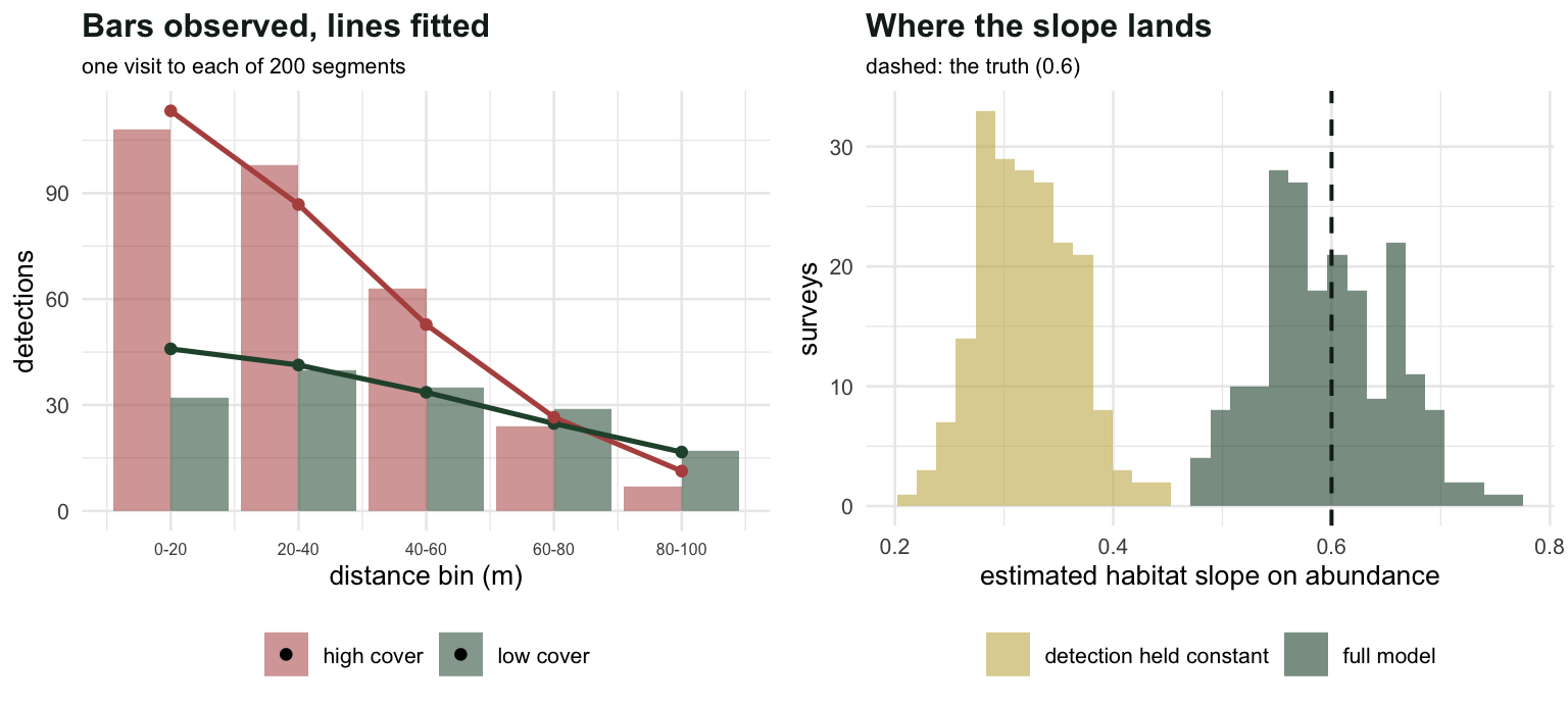
At `r sprintf("%.0f", 100*sum(d$y)/sum(d$N))` per cent detected, this is not a hard survey by the standards of the literature. Now fit the full model, and fit the version that models abundance carefully and treats detection as a constant.
```{r fits}
f4 <- fit(c(1, 0.5, log(0.05), -0.3), y = d$y, z = d$z)
f3 <- fit(c(1, 0.5, log(0.05)), y = d$y, z = d$z, sig_cov = FALSE)
rbind(FULL  = c(b0 = f4$par[1], b1 = f4$par[2], a0 = f4$par[3], a1 = f4$par[4]),
      truth = c(b0, b1, a0, a1))
sprintf("FULL : b1 %.4f (SE %.4f) | a1 %.4f (SE %.4f) | N total %.0f (true %d, raw count %d)",
        f4$par[2], f4$se[2], f4$par[4], f4$se[4],
        sum(exp(f4$par[1] + f4$par[2]*d$z)), sum(d$N), sum(d$y))
sprintf("NAIVE: b1 %.4f (SE %.4f, %+.1f%%) | 95%% CI [%.3f, %.3f] contains 0.6? %s | dAIC %.1f",
        f3$par[2], f3$se[2], 100*(f3$par[2]/b1 - 1),
        f3$par[2] - 1.96*f3$se[2], f3$par[2] + 1.96*f3$se[2],
        f3$par[2] - 1.96*f3$se[2] < b1 && b1 < f3$par[2] + 1.96*f3$se[2],
        (2*f3$nll + 6) - (2*f4$nll + 8))
```
One visit. Not three, not a mark, not a second observer: one pass with a rangefinder, and both the abundance slope and the detection slope come back with usable standard errors.
The naive model returns a habitat effect `r sprintf("%.0f", abs(100*(f3$par[2]/b1 - 1)))` per cent too small, with a confidence interval that excludes the truth. This is the [pooling trade](../covariates-in-the-detection-function/) in hierarchical clothing: detection falls where density rises, and a model with nowhere to put the detection effect books it as fewer animals.
## The exact version of that
One survey is one draw. The asymptotic value the naive slope converges to can be computed directly, by maximising the expected log-likelihood under the true world over a grid of $z$.
```{r pseudo-true}
zg <- seq(-5, 5, length.out = 601); wz <- dnorm(zg); wz <- wz/sum(wz)
Ey <- t(sapply(seq_along(zg), function(i) exp(b0 + b1*zg[i])*pi_b(exp(a0 + a1*zg[i]))))
negQ <- function(p, sig_cov = FALSE) {
  lm_ <- exp(p[1] + p[2]*zg)
  sg  <- if (sig_cov) exp(p[3] + p[4]*zg) else rep(exp(p[3]), length(zg))
  M <- t(sapply(seq_along(zg), function(i) lm_[i]*pi_b(sg[i])))
  Q <- Ey*log(M); Q[Ey == 0] <- 0        # 0 log 0 = 0, else the truth scores as undefined
  -sum(wz * rowSums(Q - M))
}
tight <- function(par, ...) {
  o <- optim(par, negQ, ..., method = "Nelder-Mead",
             control = list(reltol = 1e-14, maxit = 5000))
  for (i in 1:2) o <- optim(o$par, negQ, ..., method = "Nelder-Mead",
                            control = list(reltol = 1e-14, maxit = 5000))
  o$par
}
o4 <- tight(c(1, 0.5, log(0.05), -0.3), sig_cov = TRUE)
o3 <- tight(c(1, 0.5, log(0.05)))
sprintf("FULL model recovers the truth: largest error %.1e", max(abs(o4 - c(b0, b1, a0, a1))))
sprintf("NAIVE converges to: b1 %.4f (truth %.2f, %+.1f%%) | sigma %.5f (true range %.4f to %.4f)",
        o3[2], b1, 100*(o3[2]/b1 - 1), exp(o3[3]), exp(a0 + a1*2), exp(a0 - a1*2))
sprintf("implied mean abundance per site: truth %.4f | naive %.4f (%+.1f%%)",
        sum(wz*exp(b0 + b1*zg)), sum(wz*exp(o3[1] + o3[2]*zg)),
        100*(sum(wz*exp(o3[1] + o3[2]*zg))/sum(wz*exp(b0 + b1*zg)) - 1))
```
The first line is the check, and it earned its place: the correctly specified model must recover the truth exactly, because the expected log-likelihood is maximised at the truth for every value of $z$ at once. It initially did not, by two per cent, which is how the `0 log 0` in the line above got found. A check that cannot fail is decoration.
With that fixed, the naive slope has an exact target: `r sprintf("%.4f", o3[2])`, or `r sprintf("%.0f", abs(100*(o3[2]/b1 - 1)))` per cent low. Note what is *not* badly wrong: mean abundance is out by only `r sprintf("%.1f", abs(100*(sum(wz*exp(o3[1] + o3[2]*zg))/sum(wz*exp(b0 + b1*zg)) - 1)))` per cent. The total survives, the covariate does not, which is the same shape of damage as pooling a detection function across strata, arriving from a different direction.
```{r mc-coverage}
M <- 200
r <- t(sapply(1:M, function(i) {
  dd <- sim_hds(52830 + i)
  a <- fit(c(1, 0.5, log(0.05), -0.3), y = dd$y, z = dd$z)
  b <- fit(c(1, 0.5, log(0.05)), y = dd$y, z = dd$z, sig_cov = FALSE)
  c(a$par[2], a$se[2], b$par[2], b$se[2],
    sum(exp(a$par[1] + a$par[2]*dd$z))/sum(dd$N),
    sum(exp(b$par[1] + b$par[2]*dd$z))/sum(dd$N))
}))
cvg <- function(e, se) mean(abs(e - b1) < 1.96*se)
sprintf("FULL : b1 %.4f (SD %.4f, mean SE %.4f) | CI coverage %.3f | N_hat/N %.4f",
        mean(r[, 1]), sd(r[, 1]), mean(r[, 2]), cvg(r[, 1], r[, 2]), mean(r[, 5]))
sprintf("NAIVE: b1 %.4f (SD %.4f, mean SE %.4f) | CI coverage %.3f | N_hat/N %.4f",
        mean(r[, 3]), sd(r[, 3]), mean(r[, 4]), cvg(r[, 3], r[, 4]), mean(r[, 6]))
```
The naive slope lands on its asymptotic target of `r sprintf("%.3f", o3[2])` with a standard deviation of `r sprintf("%.3f", sd(r[, 3]))`, and a nominal 95 per cent interval covers the truth in `r sprintf("%.0f", M*cvg(r[, 3], r[, 4]))` out of `r M` surveys. Not a low coverage: zero. The intervals are the right width for a quantity that is not the one in the title.
```{r fig-fit}
#| echo: false
#| fig-width: 8
#| fig-height: 3.6
#| fig-cap: "Left: observed bin counts against the fitted expectations from the full model, split by whether the site sits above or below the covariate mean. Right: two hundred surveys, showing where each model's habitat slope lands."
#| fig-alt: "Left panel shows observed and fitted distance bin counts for low and high covariate sites, with the high sites having a steeper decline. Right panel shows two histograms of the estimated habitat slope, the full model centred on 0.6 and the naive model centred near 0.32."
ink <- "#16241d"; forest <- "#275139"; gold <- "#c9b458"; rust <- "#b5534e"
hi <- d$z > 0
obs <- rbind(data.frame(bin = 1:B, n = colSums(d$y[!hi, ]), k = "low cover", src = "observed"),
data.frame(bin = 1:B, n = colSums(d$y[hi, ]), k = "high cover", src = "observed"))
lam_h <- exp(f4$par[1] + f4$par[2]*d$z); sg_h <- exp(f4$par[3] + f4$par[4]*d$z)
Efit <- t(sapply(seq_len(R), function(i) lam_h[i]*pi_b(sg_h[i])))
fitd <- rbind(data.frame(bin = 1:B, n = colSums(Efit[!hi, ]), k = "low cover", src = "fitted"),
data.frame(bin = 1:B, n = colSums(Efit[hi, ]), k = "high cover", src = "fitted"))
p1 <- ggplot(obs, aes(bin, n, fill = k)) +
geom_col(position = "dodge", alpha = 0.55) +
geom_line(data = fitd, aes(bin, n, colour = k), linewidth = 0.9) +
geom_point(data = fitd, aes(bin, n, colour = k), size = 1.6) +
scale_fill_manual(values = c("low cover" = forest, "high cover" = rust)) +
scale_colour_manual(values = c("low cover" = forest, "high cover" = rust), guide = "none") +
scale_x_continuous(breaks = 1:B, labels = paste0(cut[-6]*1000, "-", cut[-1]*1000)) +
labs(x = "distance bin (m)", y = "detections", fill = NULL,
title = "Bars observed, lines fitted",
subtitle = "one visit to each of 200 segments") +
theme_minimal(base_size = 10) + te_canvas +
theme(legend.position = "bottom", plot.title = element_text(colour = ink, face = "bold"),
plot.subtitle = element_text(size = 8), axis.text.x = element_text(size = 6))
p2 <- ggplot(rbind(data.frame(v = r[, 1], k = "full model"),
data.frame(v = r[, 3], k = "detection held constant")),
aes(v, fill = k)) +
geom_histogram(bins = 32, position = "identity", alpha = 0.6) +
geom_vline(xintercept = b1, colour = ink, linetype = 2, linewidth = 0.7) +
scale_fill_manual(values = c("full model" = forest, "detection held constant" = gold)) +
labs(x = "estimated habitat slope on abundance", y = "surveys", fill = NULL,
title = "Where the slope lands", subtitle = "dashed: the truth (0.6)") +
theme_minimal(base_size = 10) + te_canvas +
theme(legend.position = "bottom", plot.title = element_text(colour = ink, face = "bold"),
plot.subtitle = element_text(size = 8))
grid::grid.newpage()
grid::pushViewport(grid::viewport(layout = grid::grid.layout(1, 2)))
print(p1, vp = grid::viewport(layout.pos.row = 1, layout.pos.col = 1))
print(p2, vp = grid::viewport(layout.pos.row = 1, layout.pos.col = 2))
```
## One visit with distances against three visits of counts
Now the comparison that decides which survey to run. Same sites, same abundance model, detection held constant at $\sigma = 0.03$ so that the two designs are estimating the same thing. The distance sampler visits each site once and measures. The N-mixture surveyor visits three times and counts.
```{r head-to-head-setup}
s0 <- 0.03; Tv <- 3
pbar <- mu_hn(s0, w)/w
Eg2  <- mu_hn(s0/sqrt(2), w)/w          # E[g^2] under x ~ U(0, w)
sprintf("per-visit detection probability p = mu/w = %.5f", pbar)
sprintf("but g(x) across individuals: mean %.4f, SD %.4f -> intra-class correlation %.4f",
        pbar, sqrt(Eg2 - pbar^2), (Eg2 - pbar^2)/(pbar*(1 - pbar)))
```
That second line is the whole comparison. The N-mixture model assumes every animal at a site is detected with the same probability $p$ on every visit. In a spatial world there is no such thing as *the* detection probability: an animal on the transect line is seen every time, an animal at 90 m is almost never seen, and the spread across individuals is enormous.
Whether that breaks the N-mixture depends on something the counts cannot tell you. If the animals hold their positions between visits, as territorial birds do, then each animal carries its own fixed detection probability and the counts are far too consistent between visits. If they shuffle, each animal draws a fresh distance every visit, and the marginal count is exactly $\text{Binomial}(N, \bar{p})$ with $\bar{p} = E[g]$: the N-mixture's assumption holds exactly. Both worlds have the same animals, the same detection function and the same expected count.
```{r head-to-head}
sim_world <- function(seed, territorial) {
  set.seed(seed)
  z <- rnorm(R); N <- rpois(R, exp(b0 + b1*z))
  y1 <- matrix(0, R, B); cnt <- matrix(0, R, Tv)
  for (i in seq_len(R)) {
    if (N[i] == 0) next
    x <- runif(N[i], 0, w)                    # where the animals are
    for (t in seq_len(Tv)) {
      xt  <- if (territorial) x else runif(N[i], 0, w)
      det <- runif(N[i]) < g_hn(xt, s0)
      cnt[i, t] <- sum(det)
      if (t == 1) y1[i, ] <- tabulate(findInterval(xt[det], cut, rightmost.closed = TRUE), B)
    }
  }
  list(y1 = y1, cnt = cnt, z = z, N = N)
}
## N-mixture likelihood: the binomial coefficients do not move during the fit, so build once
nmix_setup <- function(cnt, Kmax = 90) {
  Ng <- 0:Kmax
  list(logC = sapply(Ng, function(N) rowSums(lchoose(N, cnt))),
       n = rowSums(cnt), Tv = ncol(cnt),
       Nmat = matrix(Ng, nrow(cnt), Kmax + 1, byrow = TRUE))
}
nll_nmix <- function(p, S, z) {
  lam <- exp(p[1] + p[2]*z); pp <- plogis(p[3])
  LP <- dpois(S$Nmat, lam, log = TRUE) + S$logC +
        S$n*log(pp) + (S$Tv*S$Nmat - S$n)*log1p(-pp)
  -sum(log(rowSums(exp(LP))))
}
run <- function(seed, territorial) {
  dw <- sim_world(seed, territorial)
  fh <- fit(c(1, 0.5, log(0.04)), y = dw$y1, z = dw$z, sig_cov = FALSE)
  S  <- nmix_setup(dw$cnt)
  fn <- optim(c(1, 0.5, qlogis(0.4)), nll_nmix, S = S, z = dw$z, method = "Nelder-Mead")
  fn <- optim(fn$par, nll_nmix, S = S, z = dw$z, method = "Nelder-Mead")
  c(hds_b1 = fh$par[2], hds_N = sum(exp(fh$par[1] + fh$par[2]*dw$z))/sum(dw$N),
    nm_b1 = fn$par[2], nm_p = plogis(fn$par[3]),
    nm_N = sum(exp(fn$par[1] + fn$par[2]*dw$z))/sum(dw$N),
    n1 = sum(dw$y1), n3 = sum(dw$cnt),
    vv = mean(apply(dw$cnt, 1, var)))
}
for (terr in c(TRUE, FALSE)) {
  a <- run(4282, terr)
  cat(sprintf("\n--- %s world (seed 4282): %.0f detections in 1 visit, %.0f across 3 visits\n",
              if (terr) "TERRITORIAL: animals hold position" else "MOBILE: animals redraw position",
              a["n1"], a["n3"]))
  cat(sprintf("    distances, 1 visit : b1 %.4f | N_hat/N %.4f\n", a["hds_b1"], a["hds_N"]))
  cat(sprintf("    counts, 3 visits   : b1 %.4f | p_hat %.4f (true %.4f) | N_hat/N %.4f\n",
              a["nm_b1"], a["nm_p"], pbar, a["nm_N"]))
}
```
```{r head-to-head-mc}
M2 <- 100
mc <- lapply(c(TRUE, FALSE), function(terr)
  t(sapply(1:M2, function(i) run(52840 + i + 1000*terr, terr))))
names(mc) <- c("territorial", "mobile")
for (k in names(mc)) {
  x <- mc[[k]]
  cat(sprintf("\n%s world, %d surveys: %.0f detections in 1 visit vs %.0f across 3\n",
              k, M2, mean(x[, "n1"]), mean(x[, "n3"])))
  cat(sprintf("  distances, 1 visit : b1 %.4f (SD %.4f) | N_hat/N %.4f (SD %.4f)\n",
              mean(x[, "hds_b1"]), sd(x[, "hds_b1"]), mean(x[, "hds_N"]), sd(x[, "hds_N"])))
  cat(sprintf("  counts, 3 visits   : b1 %.4f (SD %.4f) | p_hat %.4f | N_hat/N %.4f (SD %.4f)\n",
              mean(x[, "nm_b1"]), sd(x[, "nm_b1"]), mean(x[, "nm_p"]),
              mean(x[, "nm_N"]), sd(x[, "nm_N"])))
}
sprintf("mean within-site variance across the 3 visits: territorial %.4f | mobile %.4f",
        mean(mc$territorial[, "vv"]), mean(mc$mobile[, "vv"]))
sprintf("territorial N_hat/N should be pbar/p_hat = %.4f; simulated %.4f",
        pbar/mean(mc$territorial[, "nm_p"]), mean(mc$territorial[, "nm_N"]))
```
Three results, and only the first one is the one people expect.
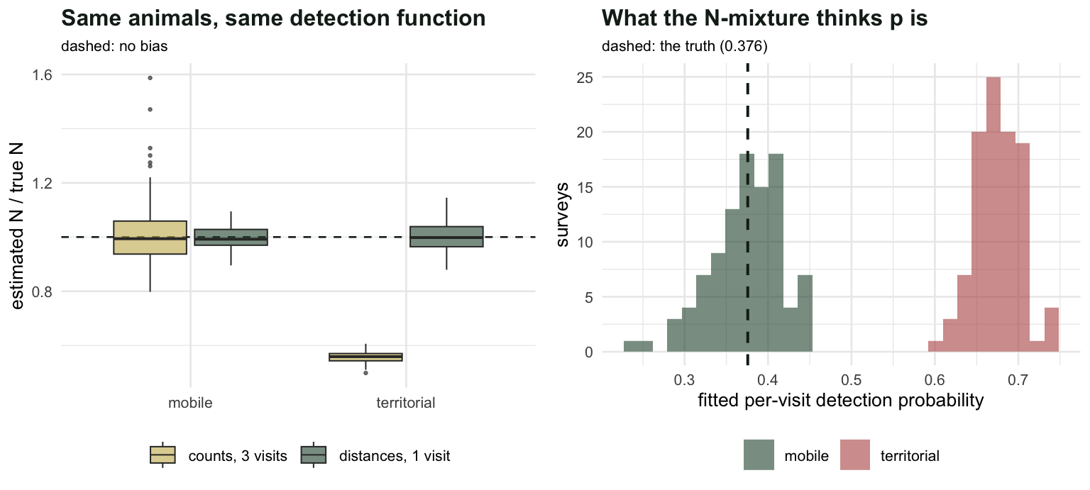
**The N-mixture loses `r sprintf("%.0f", 100*(1 - mean(mc$territorial[, "nm_N"])))` per cent of the population in the territorial world**, and it loses it upwards: the fitted detection probability comes out at `r sprintf("%.3f", mean(mc$territorial[, "nm_p"]))` against a truth of `r sprintf("%.3f", pbar)`. The mechanism is the within-site variance in the second-last line. When animals hold still, the same birds are detected every visit and the counts barely move between visits, `r sprintf("%.2f", mean(mc$territorial[, "vv"]))` against `r sprintf("%.2f", mean(mc$mobile[, "vv"]))`. Consistency is what a binomial reads as high detection, and high detection means there is nothing much left to find. The arithmetic is closed: $\hat{N}/N \to \bar{p}/\hat{p}$, which is `r sprintf("%.4f", pbar/mean(mc$territorial[, "nm_p"]))` against a simulated `r sprintf("%.4f", mean(mc$territorial[, "nm_N"]))`.
Note the direction. This is the old model-Mh result in new clothing: unmodelled individual heterogeneity in capture-recapture makes the average capture probability look higher than it is, so the abundance estimate comes out low. What decides whether it bites here is the trigger, not the heterogeneity itself: it has to be fixed across visits rather than resampled within them, which is what the between-visit variance is measuring.
**Even in the mobile world, where the N-mixture is unbiased, it is `r sprintf("%.1f", sd(mc$mobile[, "nm_N"])/sd(mc$mobile[, "hds_N"]))` times noisier**, with three times the detections. Here, with a per-visit detection probability near `r sprintf("%.2f", pbar)` and three visits, repeat visits were an expensive way to buy detection, because they measure it indirectly through a variance.
**The habitat slope is fine everywhere**, near `r sprintf("%.2f", mean(mc$mobile[, "nm_b1"]))` in all four cells. A detection bias that is constant across sites moves the intercept and leaves the slope alone. If your paper is about which habitat has more birds, the N-mixture will not embarrass you. If a number of animals appears in the abstract, it might.
```{r fig-h2h}
#| echo: false
#| fig-width: 8
#| fig-height: 3.6
#| fig-cap: "One hundred surveys in each world. Left: estimated abundance as a fraction of the truth. Right: the fitted per-visit detection probability, which is what the N-mixture gets wrong when animals hold still."
#| fig-alt: "Left panel shows abundance ratios: distance sampling sits on one in both worlds, while the N-mixture sits on one in the mobile world and near 0.56 in the territorial world. Right panel shows the fitted detection probability, correct in the mobile world and inflated in the territorial world."
dfN <- do.call(rbind, lapply(names(mc), function(k) rbind(
data.frame(v = mc[[k]][, "hds_N"], world = k, m = "distances, 1 visit"),
data.frame(v = mc[[k]][, "nm_N"], world = k, m = "counts, 3 visits"))))
p1 <- ggplot(dfN, aes(world, v, fill = m)) +
geom_hline(yintercept = 1, colour = ink, linetype = 2) +
geom_boxplot(alpha = 0.6, outlier.size = 0.5, linewidth = 0.35) +
scale_fill_manual(values = c("distances, 1 visit" = forest, "counts, 3 visits" = gold)) +
labs(x = NULL, y = "estimated N / true N", fill = NULL,
title = "Same animals, same detection function",
subtitle = "dashed: no bias") +
theme_minimal(base_size = 10) + te_canvas +
theme(legend.position = "bottom", plot.title = element_text(colour = ink, face = "bold"),
plot.subtitle = element_text(size = 8))
dfp <- do.call(rbind, lapply(names(mc), function(k)
data.frame(v = mc[[k]][, "nm_p"], world = k)))
p2 <- ggplot(dfp, aes(v, fill = world)) +
geom_histogram(bins = 30, position = "identity", alpha = 0.6) +
geom_vline(xintercept = pbar, colour = ink, linetype = 2, linewidth = 0.7) +
scale_fill_manual(values = c(territorial = rust, mobile = forest)) +
labs(x = "fitted per-visit detection probability", y = "surveys", fill = NULL,
title = "What the N-mixture thinks p is",
subtitle = sprintf("dashed: the truth (%.3f)", pbar)) +
theme_minimal(base_size = 10) + te_canvas +
theme(legend.position = "bottom", plot.title = element_text(colour = ink, face = "bold"),
plot.subtitle = element_text(size = 8))
grid::grid.newpage()
grid::pushViewport(grid::viewport(layout = grid::grid.layout(1, 2)))
print(p1, vp = grid::viewport(layout.pos.row = 1, layout.pos.col = 1))
print(p2, vp = grid::viewport(layout.pos.row = 1, layout.pos.col = 2))
```
```{r}
#| label: thumb
#| include: false
thumb_title <- paste(strwrap("Same animals, same detection function", 46), collapse = "\n")
ggsave("thumbnail.png",
p1 + labs(title = thumb_title) +
theme(plot.title = element_text(size = 13, face = "bold"),
plot.subtitle = element_text(size = 9.5),
plot.margin = margin(8, 14, 8, 8)),
width = 7.5, height = 5.4, dpi = 100, bg = "#f5f4ee")
```
## What this does not fix
The comparison above is not a claim that distance sampling is the better method. It is a claim that the two designs bet on different biology, and that the bets are worth stating out loud.
The N-mixture bets that your animals shuffle between visits, or near enough that a common $p$ is a fair summary. For a territorial songbird in June that bet is poor, and Barker et al. (2018) show the same family of failures from several directions. For a foraging flock it may be fine.
Hierarchical distance sampling bets instead that animals are uniformly distributed with respect to the transect, that everything on the line is detected, and that they hold still *within* a visit rather than moving in response to you. Those are different assumptions, not weaker ones. They are also mostly design choices: random placement makes the first one true by construction, which is why it is worth being fussy about.
And the model still leans on its abundance distribution. The independent-Poisson identity that makes the likelihood two lines long is exactly the property that fails under a negative binomial, so extra-Poisson variation in abundance has to be added back by hand. For the negative binomial that can still be done in closed form, because the total count at a site is then negative binomial with mean $\lambda_s \sum_b \pi_b$ and the same size, and the split of that total across the bins is multinomial; other abundance distributions have to be worked out one at a time, and for some of them the latent-N sum returns along with its truncation ceiling. Sillett et al. (2012) work a full hierarchical distance sampling analysis on an island endemic and are explicit about which of these are assumptions and which are protocol.
The [closing post](../checking-a-distance-sampling-model/) asks what a fitted detection function will actually tell you when one of these is wrong, and the answer is worse than you would guess.
## References
Barker RJ, Schofield MR, Link WA, Sauer JR 2018 Biometrics 74(1):369-377 (10.1111/biom.12734)
Buckland ST, Rexstad EA, Marques TA, Oedekoven CS 2015 Distance Sampling: Methods and Applications. Springer. ISBN 978-3-319-19218-5
Kery M, Royle JA 2016 Applied Hierarchical Modeling in Ecology. Academic Press. ISBN 978-0-12-801378-6
Royle JA 2004 Biometrics 60(1):108-115 (10.1111/j.0006-341X.2004.00142.x)
Royle JA, Dawson DK, Bates S 2004 Ecology 85(6):1591-1597 (10.1890/03-3127)
Sillett TS, Chandler RB, Royle JA, Kery M, Morrison SA 2012 Ecological Applications 22(7):1997-2006 (10.1890/11-1400.1)
## Related tutorials
- [N-mixture models for abundance](../n-mixture-models-abundance/)
- [Detection from a single drone flight](../detection-from-a-single-flight/)
- [Point transect distance sampling](../point-transect-distance-sampling/)
- [Checking a distance sampling model](../checking-a-distance-sampling-model/)