Distance sampling for density in R

Estimate animal density from line-transect surveys when detection falls with distance. Fit half-normal and hazard-rate detection functions from scratch in R.

Walk a line through a study area and record every animal you see, along with how far off the line it was. Close to the line you miss almost nothing; far from it you miss most things. If you simply counted everything within a fixed strip and divided by the strip area, you would treat those distant misses as absences and report a density well below the truth.

Distance sampling fixes this by modelling how detection falls with distance. The shape of that decline, estimated from the perpendicular distances themselves, tells you what fraction of animals in the strip you actually saw, and dividing by that fraction recovers the real density. This post fits the half-normal and hazard-rate detection functions by hand with optim, turns each into a density estimate, and uses AIC to choose between them.

The idea

Suppose animals are spread at random through a strip of half-width w on each side of the line, and an animal at perpendicular distance x is detected with probability g(x), where g(0) = 1 and g falls with distance. The perpendicular distances of the animals you do detect have probability density

\[f(x) = \frac{g(x)}{\mu}, \qquad \mu = \int_0^{w} g(x)\, dx,\]

where mu is the effective strip half-width. It is the width of a strip that, if every animal in it were seen and none outside, would give the same expected count. The average detection probability inside w is then mu / w. If n animals are detected along a line of length L, the density is

\[\hat{D} = \frac{n}{2 L \hat{\mu}},\]

with the factor of two for the two sides of the line. All the work is in estimating mu, which means estimating the detection function.

Simulating a line-transect survey

We survey 30 km of line with a truncation distance of 0.15 km. The true detection follows a half-normal with scale 0.06 km, and the true density is 80 animals per square kilometre. We place the animals in the strip, then keep each with a probability that falls with distance.

library(ggplot2)
library(dplyr)

ink <- "#16241d"; body <- "#2c3a31"; forest <- "#275139"; gold <- "#c9b458"
paper <- "#f5f4ee"; line_c <- "#dad9ca"; faint <- "#5d6b61"; sage <- "#93a87f"; red <- "#b5534e"

theme_te <- function(base = 12) {
  theme_minimal(base_size = base) +
    theme(panel.grid.minor = element_blank(),
          panel.grid.major = element_line(colour = line_c, linewidth = 0.3),
          plot.background = element_rect(fill = paper, colour = NA),
          panel.background = element_rect(fill = paper, colour = NA),
          axis.title = element_text(colour = body), axis.text = element_text(colour = faint),
          plot.title = element_text(colour = ink, face = "bold"),
          plot.subtitle = element_text(colour = faint),
          legend.title = element_text(colour = body), legend.text = element_text(colour = faint))
}

set.seed(6)
Dtrue <- 80; L <- 30; w <- 0.15; sig_true <- 0.06

area <- 2 * w * L                 # surveyed strip area
Ntot <- round(Dtrue * area)       # animals present in the strip
xall <- runif(Ntot, 0, w)         # perpendicular distances, uniform in the strip
det <- rbinom(Ntot, 1, exp(-xall^2 / (2 * sig_true^2)))   # detected with prob g(x)
x <- xall[det == 1]               # distances of detected animals
nobs <- length(x)
c(present = Ntot, detected = nobs)

 present detected 
     720      362 

Of the 720 animals in the strip, 362 are detected. The rest were present but missed, mostly out toward the truncation distance.

The naive strip estimate

Divide the detections by the strip area, as if detection were perfect, and the density comes out far too low.

D_naive <- nobs / (2 * w * L)
c(D_naive = D_naive, D_true = Dtrue)

 D_naive   D_true 
40.22222 80.00000 

The naive estimate is 40 animals per square kilometre, almost exactly half the true 80, because about half the animals in the strip went undetected. Distance sampling recovers the missing half from the shape of the distance histogram.

Fitting the half-normal detection function

The half-normal is g(x) = exp(-x^2 / (2 sigma^2)). Its effective strip half-width has a closed form through the normal distribution function, so the likelihood needs only optim over the log scale.

mu_hn <- function(s) s * sqrt(2 * pi) * (pnorm(w / s) - 0.5)   # integral of g over [0, w]
nll_hn <- function(ls) {
  s <- exp(ls)
  -sum(-x^2 / (2 * s^2) - log(mu_hn(s)))   # f(x) = g(x) / mu
}
ohn <- optim(log(0.05), nll_hn, method = "BFGS", hessian = TRUE)
sig <- exp(ohn$par); mu <- mu_hn(sig)
Phat <- mu / w
c(sigma_hat = sig, ESW = mu, detection_prob = Phat)

     sigma_hat            ESW detection_prob 
    0.06111697     0.07551753     0.50345022 

The scale is estimated at 0.061 km, close to the true 0.06, giving an effective strip half-width of 0.076 km. That is only about half the truncation width, so the average detection probability inside the strip is 0.50: the survey saw half of what was there, which is what the naive estimate missed.

g_hr <- function(xx, s, b) 1 - exp(-(xx / s)^(-b))          # hazard-rate detection
mu_hr <- function(s, b) integrate(function(u) g_hr(u, s, b), 0, w)$value
nll_hr <- function(par) {
  s <- exp(par[1]); b <- exp(par[2]); m <- mu_hr(s, b)
  if (!is.finite(m) || m <= 0) return(1e6)
  -sum(log(g_hr(x, s, b)) - log(m))
}
ohr <- optim(c(log(0.06), log(3)), nll_hr, method = "BFGS", hessian = TRUE)
shr <- exp(ohr$par[1]); bhr <- exp(ohr$par[2]); muhr <- mu_hr(shr, bhr)

xs <- seq(0, w, length.out = 200)
fhn <- exp(-xs^2 / (2 * sig^2)) / mu
fhr <- g_hr(xs, shr, bhr) / muhr
dfit <- data.frame(x = rep(xs, 2), f = c(fhn, fhr),
                   model = rep(c("Half-normal", "Hazard-rate"), each = length(xs)))

ggplot(data.frame(x = x), aes(x)) +
  geom_histogram(aes(y = after_stat(density)), breaks = seq(0, w, by = 0.015),
                 fill = sage, colour = paper, linewidth = 0.3) +
  geom_line(data = dfit, aes(x, f, colour = model), linewidth = 0.9) +
  scale_colour_manual(values = c("Half-normal" = forest, "Hazard-rate" = red), name = NULL) +
  labs(title = "Detected objects thin out with distance",
       subtitle = "Perpendicular-distance histogram with fitted detection functions",
       x = "Perpendicular distance (km)", y = "Probability density") +
  theme_te() + theme(legend.position = c(0.82, 0.82))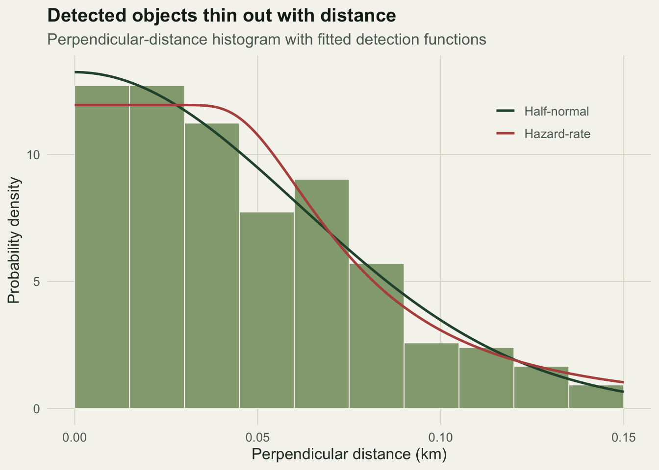

Figure 1: Perpendicular-distance histogram of detected animals with the fitted half-normal and hazard-rate detection densities.

From detection function to density

The effective strip half-width folds the whole detection curve into a single width. A rectangle of height one and width mu has the same area as the region under the detection function, which is what makes the density formula work.

gcurve <- data.frame(x = xs, g = exp(-xs^2 / (2 * sig^2)))
ggplot(gcurve, aes(x, g)) +
  annotate("rect", xmin = 0, xmax = mu, ymin = 0, ymax = 1, fill = gold, alpha = 0.25) +
  geom_line(colour = forest, linewidth = 0.9) +
  geom_vline(xintercept = w, linetype = "dashed", colour = faint) +
  annotate("text", x = mu, y = 0.5, label = sprintf("ESW = %.3f km", mu),
           colour = ink, hjust = -0.05, size = 3.4) +
  annotate("text", x = w, y = 0.95, label = "truncation w", colour = faint, hjust = 1.05, size = 3.2) +
  labs(title = "Effective strip half-width folds detection into an area",
       subtitle = "Fitted half-normal detection function; the shaded rectangle has the same area",
       x = "Perpendicular distance (km)", y = "Detection probability") +
  theme_te()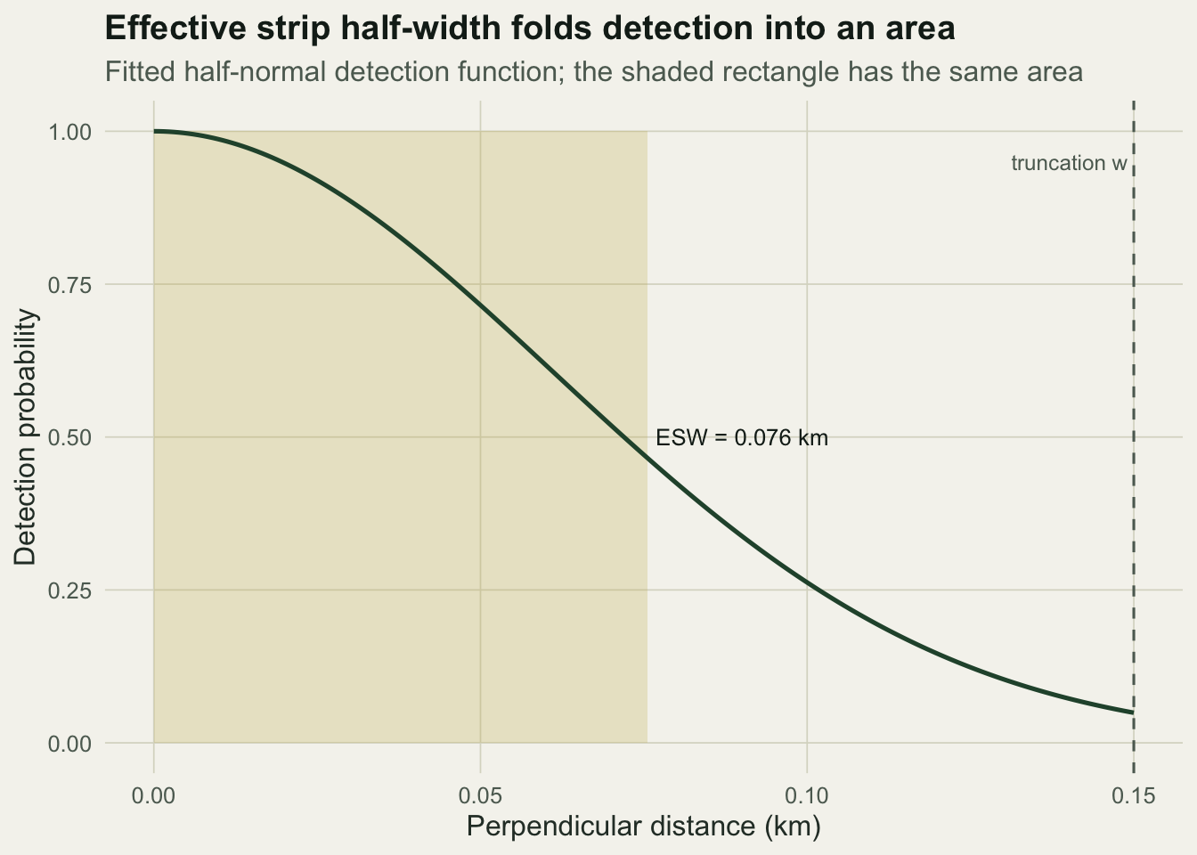

Figure 2: Fitted half-normal detection function with the effective strip half-width drawn as an equal-area rectangle.

The density estimate combines the encounter rate with this width, and its uncertainty has two parts: the sampling variation in the number seen, and the uncertainty in the fitted detection function.

D_hat <- nobs / (2 * L * mu)
se_ls <- sqrt(1 / ohn$hessian[1, 1])                  # SE of log sigma
eps <- 1e-5
dlogmu <- (log(mu_hn(exp(ohn$par + eps))) - log(mu_hn(exp(ohn$par - eps)))) / (2 * eps)
cv2 <- 1 / nobs + (dlogmu * se_ls)^2                  # encounter rate plus detection function
se_D <- D_hat * sqrt(cv2)
D_ci <- D_hat + c(-1.96, 1.96) * se_D
round(c(D_hat = D_hat, se = se_D, lo = D_ci[1], hi = D_ci[2], true = Dtrue), 1)

D_hat    se    lo    hi  true 
 79.9   5.4  69.4  90.4  80.0 

d3 <- data.frame(
  est = factor(c("Naive: assume\nperfect detection", "Distance sampling\nD-hat", "Truth"),
               levels = c("Naive: assume\nperfect detection", "Distance sampling\nD-hat", "Truth")),
  val = c(D_naive, D_hat, Dtrue), lo = c(NA, D_ci[1], NA), hi = c(NA, D_ci[2], NA),
  fill = c("naive", "model", "truth"))
ggplot(d3, aes(est, val, fill = fill)) +
  geom_col(width = 0.6) +
  geom_errorbar(aes(ymin = lo, ymax = hi), width = 0.15, colour = ink, na.rm = TRUE) +
  geom_hline(yintercept = Dtrue, linetype = "dashed", colour = faint, linewidth = 0.4) +
  scale_fill_manual(values = c(naive = gold, model = forest, truth = sage), guide = "none") +
  labs(title = "Ignoring imperfect detection halves the density",
       subtitle = "Estimated density: naive strip count versus distance sampling",
       x = NULL, y = "Objects per square km") +
  theme_te()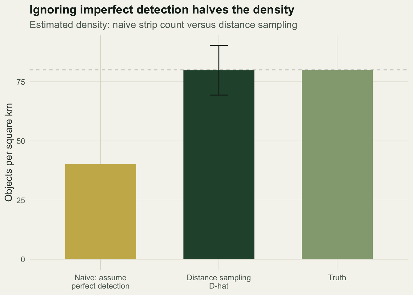

Figure 3: Density estimates: the naive strip count assuming perfect detection, and the distance-sampling estimate with its 95% interval, against the truth.

The distance-sampling estimate is 80 animals per square kilometre with a 95% interval of about 69 to 90, recovering the true density that the naive strip count halved.

Choosing the detection function

We fitted a hazard-rate function as well, which has a flatter shoulder near the line and a sharper drop beyond. AIC compares the two, penalising the hazard-rate for its extra parameter.

ll_hn <- -ohn$value; ll_hr <- -ohr$value
aic_hn <- -2 * ll_hn + 2 * 1
aic_hr <- -2 * ll_hr + 2 * 2
c(AIC_half_normal = aic_hn, AIC_hazard_rate = aic_hr, difference = aic_hr - aic_hn)

AIC_half_normal AIC_hazard_rate      difference 
   -1541.734462    -1538.647743        3.086719 

The half-normal wins by about three AIC units, which is the right answer since the data were generated from a half-normal and the hazard-rate’s second parameter buys no real improvement. On field data the choice matters more, because a detection function that bends the wrong way near the line biases the density. Fitting several shapes and comparing them, rather than defaulting to one, is standard practice.

Assumptions and when it fails

Distance sampling rests on a few conditions. Everything on the line must be detected, so g(0) = 1; animals must be recorded at their initial location before they react to the observer; distances must be measured accurately, since rounding to convenient values distorts the histogram near the line; and the lines must be placed at random with respect to the animals, not along features like ridges or rivers that concentrate them. When detection on the line is uncertain, as for diving whales or cryptic birds, the density is biased low and a double-observer method is needed. When distances are heaped at round numbers, binning the data into distance intervals helps. The standard software (Thomas and colleagues 2010; Miller and colleagues 2019) fits these functions and their variances directly, but the mechanism is the one built by hand above.

References

Buckland, Anderson, Burnham, Laake, Borchers and Thomas 2001 Introduction to Distance Sampling (Oxford University Press, ISBN 978-0-19-850927-1)

Thomas, Buckland, Rexstad et al 2010 Journal of Applied Ecology 47(1):5-14 (10.1111/j.1365-2664.2009.01737.x)

Miller, Rexstad, Thomas, Marshall and Laake 2019 Journal of Statistical Software 89(1):1-28 (10.18637/jss.v089.i01)

Related tutorials

• N-mixture models for abundance in R
• Removal and depletion sampling in R
• Closed-population capture-recapture in R
• Model selection with AIC in R