library(ggplot2)
te_canvas <- theme(plot.background  = element_rect(fill = "#f5f4ee", colour = NA),
                   panel.background = element_rect(fill = "#f5f4ee", colour = NA))

## half-normal detection function and its effective strip half-width
g_hn  <- function(x, s) exp(-x^2/(2*s^2))
mu_hn <- function(s, w) sqrt(2*pi)*s*(pnorm(w, 0, s) - 0.5)   # integral of g from 0 to w

## log density of an observed distance, written out rather than as log(g/mu):
## g underflows to zero in the tail and log(0) would stop every integral below
ld_hn <- function(x, s, w) -x^2/(2*s^2) - log(mu_hn(s, w))

## hazard-rate key, for later
g_hr  <- function(x, s, b) 1 - exp(-(x/s)^(-b))
mu_hr <- function(s, b, w) integrate(g_hr, 0, w, s = s, b = b)$valueCovariates in the detection function
R
distance sampling
imperfect detection
abundance
ecology tutorial
Pooling one detection function across strata keeps the total density roughly right and gets the comparison between strata badly wrong. Worked in base R.
Corrected 7 October 2026: the post said the pooled hazard-rate key does slightly better on the total than the pooled half-normal; it now says it does clearly better, as its output shows.
Corrected 30 September 2026: the group size section said a cited bird survey analysis used group size and habitat as detection covariates; it now says that analysis used observer and time of day.
Corrected 27 September 2026: the highlighted summary said the pooled estimator is close to unbiased for the study area; it now says the total is roughly right but 13 per cent low here, as the output shows.
A line transect survey gives you distances, and the basic analysis turns them into a density: fit a detection function to the perpendicular distances, integrate it to get the effective strip half-width, divide the count by the area that width implies. One detection function, one density.
Almost no survey is that simple. You walk two habitats, or three observers take turns, or the animals occur in groups of one and groups of twenty. Detectability moves, and the usual advice is that it does not matter much, because the total comes out about right anyway.
The advice is half true, and the half that is false is the half most people are actually using. This post takes a survey with two strata, works out exactly what a single pooled detection function does to it, and then puts the covariate where it belongs.
A survey with two strata
Two habitats, walked with the same effort. In the open stratum the animals are easy to see; in the dense stratum they are not. The truncation distance is 100 m in both.
w   <- 0.1                    # truncation distance, km
L   <- c(open = 50, dense = 50)  # transect length per stratum, km
D   <- c(open = 30, dense = 60)  # TRUE density, groups per km2
sig <- c(open = 0.060, dense = 0.025)
area  <- 2*w*L                # covered area per stratum, km2
Ntrue <- D*area               # animals in the covered strip
mu    <- mu_hn(sig, w)        # vectorised over sigma. Writing this as
                              # c(open = mu_hn(sig["open"], w)) names the element
                              # "open.open", and mu["open"] then silently misses
Pdet  <- mu/w                 # probability of detecting an animal in the strip
En    <- 2*D*L*mu             # expected detections
data.frame(sigma = sig, mu = round(mu, 5), P_detect = round(Pdet, 4),
           N_in_strip = Ntrue, E_detections = round(En, 1))
sigma mu P_detect N_in_strip E_detections
open 0.060 0.06801 0.6801 300 204
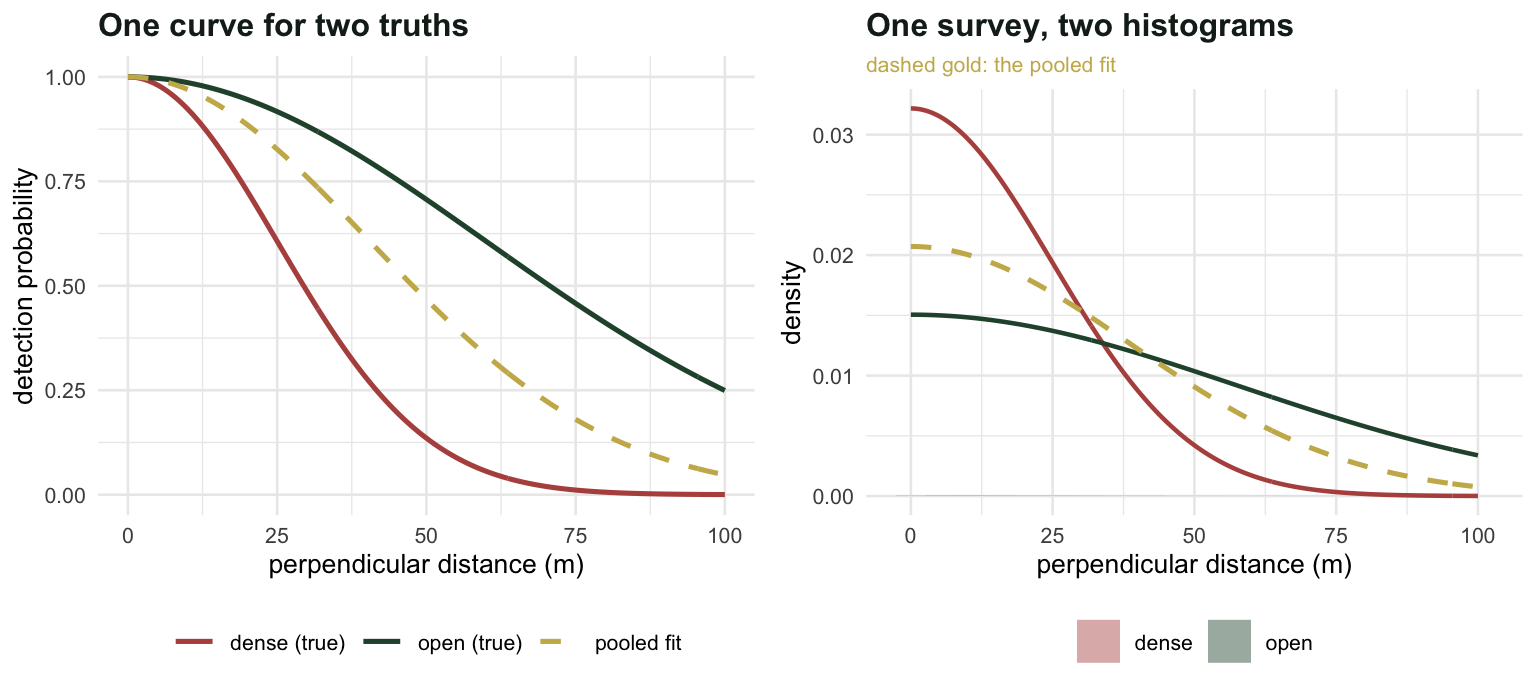
dense 0.025 0.03133 0.3133 600 188The dense stratum holds 2 times as many animals per square kilometre as the open one. It produces 188 detections against 204.
That is not a rounding artefact and it is not sampling noise: those are exact expectations. If you compare raw encounter rates, the stratum with twice the density looks like the emptier one, by a factor of 0.9213.
sprintf("naive encounter-rate ratio dense/open: %.4f   (truth: %.1f)",
        En["dense"]/En["open"], D["dense"]/D["open"])
[1] "naive encounter-rate ratio dense/open: 0.9213 (truth: 2.0)"Nobody would publish that number as a density comparison. The question is what happens when you do the respectable thing instead, and fit a detection function to all the distances at once.
What pooling actually fits
Pool the two strata and fit a single half-normal. With a large enough sample, the fitted scale converges to the value that minimises the Kullback-Leibler divergence from the true pooled distribution of distances. For the half-normal there is a shortcut: the maximum likelihood estimator solves a moment identity, so the pooled limit is the scale whose truncated second moment matches the true pooled second moment.
## true pooled density of observed distances: a mixture weighted by expected detections
wt   <- En/sum(En)
fmix <- function(x) wt["open"]*g_hn(x, sig["open"])/mu["open"] +
                    wt["dense"]*g_hn(x, sig["dense"])/mu["dense"]

## route 1: match the truncated second moment
m2_hn <- function(s, w) s^2*(1 - w*g_hn(w, s)/mu_hn(s, w))
m2_true <- integrate(function(x) x^2*fmix(x), 0, w)$value
sig_star_mom <- uniroot(function(s) m2_hn(s, w) - m2_true, c(0.005, 0.5), tol = 1e-12)$root

## route 2: minimise the KL divergence directly
kl <- function(s) -integrate(function(x) fmix(x)*ld_hn(x, s, w), 0, w)$value
sig_star_kl <- optimise(kl, c(0.005, 0.3), tol = 1e-12)$minimum

sprintf("pooled sigma*: moment identity %.7f | direct KL %.7f | difference %.2e",
        sig_star_mom, sig_star_kl, sig_star_mom - sig_star_kl)
[1] "pooled sigma*: moment identity 0.0405237 | direct KL 0.0405237 | difference -5.85e-10"The two routes agree to \(6 \times 10^{-10}\), which is the check worth having: the arithmetic below rests on this one number, so it is worth getting it from two directions.
Now push the pooled scale through the density estimator. Every animal, whichever stratum it came from, is credited with the same effective strip half-width.
mu_star <- mu_hn(sig_star_mom, w)
D_pool_total   <- sum(En)/(2*sum(L)*mu_star)
D_pool_stratum <- En/(2*L*mu_star)

data.frame(stratum = names(D),
           D_true = as.numeric(D),
           D_pooled = round(as.numeric(D_pool_stratum), 2),
           error_pct = round(100*(D_pool_stratum/D - 1), 1))
stratum D_true D_pooled error_pct
open open 30 40.73 35.8
dense dense 60 37.52 -37.5sprintf("TOTAL: true %.2f | pooled %.2f (%+.2f%%)", sum(Ntrue)/sum(area),
D_pool_total, 100*(D_pool_total/(sum(Ntrue)/sum(area)) - 1))[1] "TOTAL: true 45.00 | pooled 39.12 (-13.06%)"sprintf("STRATUM RATIO: true %.2f | pooled %.4f (%+.1f%%)",
D["dense"]/D["open"], D_pool_stratum["dense"]/D_pool_stratum["open"],
100*((D_pool_stratum["dense"]/D_pool_stratum["open"])/(D["dense"]/D["open"]) - 1))[1] "STRATUM RATIO: true 2.00 | pooled 0.9213 (-53.9%)"There it is. The total is out by 13.1 per cent, which for a wildlife survey is a bad afternoon rather than a disaster. The ratio between strata is out by 54 per cent, and worse than the size of the error is its sign: the pooled analysis says the dense stratum is emptier than the open one.
It says this because pooling cannot change the ratio at all. Both strata get divided by the same effective width, so the pooled ratio is the encounter-rate ratio from the first section, wearing a detection function as a disguise. The detection function moves both numbers together and cancels out of their ratio exactly.
The pooled estimator gets the study-area total roughly right (13 per cent low here) and gives you no protection whatsoever on any comparison inside it. Rexstad et al. (2023) make the same point with simulations and a songbird dataset: the property people rely on is a statement about the total, and it was never a statement about the parts.
The hazard-rate key, with its extra shape parameter, does clearly better on the total and exactly as badly on the ratio.
kl_hr <- function(p) {
  s <- exp(p[1]); b <- exp(p[2])
  v <- try(-integrate(function(x) fmix(x)*log(g_hr(x, s, b)/mu_hr(s, b, w)),
                      1e-6, w)$value, silent = TRUE)
  if (inherits(v, "try-error") || !is.finite(v)) 1e10 else v
}
o <- optim(c(log(0.04), log(2.5)), kl_hr, method = "Nelder-Mead",
           control = list(reltol = 1e-12))
o <- optim(o$par, kl_hr, method = "Nelder-Mead", control = list(reltol = 1e-12))
mu_hr_star <- mu_hr(exp(o$par[1]), exp(o$par[2]), w)
sprintf("hazard-rate pooled: total D %.2f (%+.2f%%) | ratio still %.4f",
        sum(En)/(2*sum(L)*mu_hr_star),
        100*(sum(En)/(2*sum(L)*mu_hr_star)/(sum(Ntrue)/sum(area)) - 1),
        En["dense"]/En["open"])
[1] "hazard-rate pooled: total D 42.34 (-5.90%) | ratio still 0.9213"More shape flexibility buys a better total. It buys nothing at all for the comparison, because the problem was never the shape of the curve.
Putting the covariate in
Multiple-covariate distance sampling (Marques and Buckland 2003) keeps the shape of the key function and lets its scale depend on covariates, on the log scale:
\[\sigma_i = \exp(\alpha_0 + \alpha_1 z_i)\]
where \(z_i\) is whatever was recorded at detection \(i\): habitat, observer, sea state, group size. The likelihood is the same conditional likelihood as before, one term per detection, except that each animal now has its own \(\sigma_i\) and therefore its own effective strip half-width \(\mu(\sigma_i)\). Density stops being one count over one width, and becomes a Horvitz-Thompson sum: every animal is credited with the area over which an animal like it could have been seen.
## exact: does the covariate model recover the truth as the sample grows?
z <- c(open = 0, dense = 1)
nll_pop <- function(p) {           # expected negative log-likelihood under the truth
  s <- exp(p[1] + p[2]*z)
  -sum(sapply(names(z), function(k)
    En[k]*integrate(function(x) (g_hn(x, sig[k])/mu[k])*ld_hn(x, s[k], w), 0, w)$value))
}
om <- optim(c(log(0.05), -0.5), nll_pop, method = "Nelder-Mead", control = list(reltol = 1e-14))
om <- optim(om$par, nll_pop, method = "Nelder-Mead", control = list(reltol = 1e-14))
s_hat <- exp(om$par[1] + om$par[2]*z)
D_mcds <- En/(2*L*mu_hn(s_hat, w))
sprintf("recovered sigma: open %.6f (true %.3f) | dense %.6f (true %.3f)",
        s_hat["open"], sig["open"], s_hat["dense"], sig["dense"])
[1] "recovered sigma: open 0.060000 (true 0.060) | dense 0.025000 (true 0.025)"sprintf("recovered D: open %.4f | dense %.4f | ratio %.6f", D_mcds["open"], D_mcds["dense"],
D_mcds["dense"]/D_mcds["open"])[1] "recovered D: open 30.0000 | dense 60.0000 | ratio 2.000000"Exactly right, which is the least a correctly specified model should manage. The point of computing it is that it fixes the target: everything below is the distance between a finite survey and this.
One survey
set.seed(4280)
sim <- function(seed = NULL) {
  if (!is.null(seed)) set.seed(seed)
  do.call(rbind, lapply(names(D), function(k) {
    x <- runif(Ntrue[k], 0, w)
    x <- x[runif(Ntrue[k]) < g_hn(x, sig[k])]
    data.frame(x = x, stratum = k, z = unname(z[k]))
  }))
}
d <- sim()
table(d$stratum)
dense  open
  200   192
## pooled fit
nll_pool <- function(p, x) -sum(ld_hn(x, exp(p), w))
fp <- optimise(function(p) nll_pool(p, d$x), c(-6, 0), tol = 1e-10)
sig_p <- exp(fp$minimum)
## covariate fit
nll_cov <- function(p, x, z) {
s <- exp(p[1] + p[2]*z)
-sum(-x^2/(2*s^2) - log(mu_hn(s, w)))
}
fc <- optim(c(log(0.04), -0.5), nll_cov, x = d$x, z = d$z, method = "Nelder-Mead")
stopifnot(fc$convergence == 0) # check before inverting the Hessian
fc <- optim(fc$par, nll_cov, x = d$x, z = d$z, method = "Nelder-Mead", hessian = TRUE)
se_a1 <- sqrt(diag(solve(fc$hessian)))[2]
n_k <- table(d$stratum)[names(D)]
Dp <- n_k/(2*L*mu_hn(sig_p, w))
sc <- exp(fc$par[1] + fc$par[2]*z)
Dc <- n_k/(2*L*mu_hn(sc, w))
dAIC <- (2*fp$objective + 2) - (2*fc$value + 4)
sprintf("n = %d open, %d dense | pooled sigma %.5f -> total D %.2f | ratio %.3f",
n_k["open"], n_k["dense"], sig_p, sum(n_k)/(2*sum(L)*mu_hn(sig_p, w)),
Dp["dense"]/Dp["open"])[1] "n = 192 open, 200 dense | pooled sigma 0.03892 -> total D 40.60 | ratio 1.042"sprintf("covariate alpha1 %.3f (SE %.3f) -> total D %.2f | ratio %.3f | dAIC %.1f",
fc$par[2], se_a1, sum(Dc*area)/sum(area), Dc["dense"]/Dc["open"], dAIC)[1] "covariate alpha1 -0.847 (SE 0.110) -> total D 46.63 | ratio 2.226 | dAIC 86.8"The covariate model wins on AIC by 87, which is not a close call, and the two analyses disagree about how much more the dense stratum holds. Pooling flattens the density ratio to 1.04, near parity; the covariate fit puts it at 2.23, close to the true 2.
Four hundred surveys
One survey is an anecdote. The question is whether the pooled analysis ever gets the comparison right, and how big the AIC signal is when it does not.
M <- 400
res <- t(sapply(1:M, function(i) {
  d <- sim(52800 + i)
  n_k <- table(factor(d$stratum, levels = names(D)))
  fp <- optimise(function(p) nll_pool(p, d$x), c(-6, 0), tol = 1e-10)
  fc <- optim(c(log(0.04), -0.5), nll_cov, x = d$x, z = d$z, method = "Nelder-Mead")
  fc <- optim(fc$par, nll_cov, x = d$x, z = d$z, method = "Nelder-Mead")
  mp <- mu_hn(exp(fp$minimum), w)
  sc <- exp(fc$par[1] + fc$par[2]*z)
  Dp <- n_k/(2*L*mp); Dc <- n_k/(2*L*mu_hn(sc, w))
  c(Dp_tot = sum(n_k)/(2*sum(L)*mp), Dc_tot = sum(Dc*area)/sum(area),
    Rp = Dp[2]/Dp[1], Rc = Dc[2]/Dc[1],
    dAIC = (2*fp$objective + 2) - (2*fc$value + 4))
}))
Dtot <- sum(Ntrue)/sum(area)
sprintf("total density (truth %.1f): pooled %.2f (SD %.2f, %+.1f%%) | covariate %.2f (SD %.2f, %+.1f%%)",
        Dtot, mean(res[, "Dp_tot"]), sd(res[, "Dp_tot"]), 100*(mean(res[, "Dp_tot"])/Dtot - 1),
        mean(res[, "Dc_tot"]), sd(res[, "Dc_tot"]), 100*(mean(res[, "Dc_tot"])/Dtot - 1))
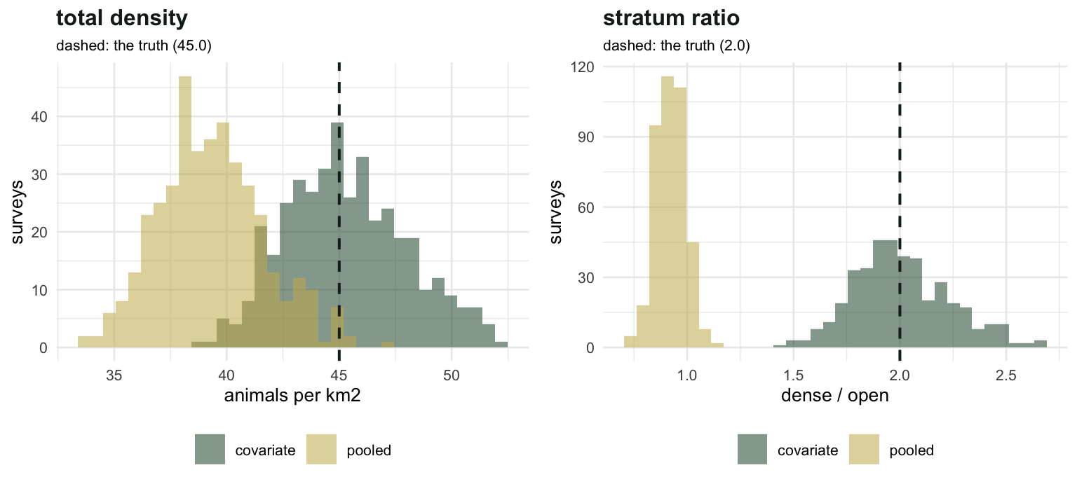
[1] "total density (truth 45.0): pooled 39.31 (SD 2.33, -12.6%) | covariate 45.30 (SD 2.69, +0.7%)"sprintf("stratum ratio (truth 2.00): pooled %.3f (SD %.3f) | covariate %.3f (SD %.3f)",
mean(res[, "Rp.dense"]), sd(res[, "Rp.dense"]),
mean(res[, "Rc.dense"]), sd(res[, "Rc.dense"]))[1] "stratum ratio (truth 2.00): pooled 0.922 (SD 0.069) | covariate 2.010 (SD 0.228)"sprintf("pooled analysis calls the dense stratum denser in %.1f%% of surveys; dAIC > 2 in %.1f%%",
100*mean(res[, "Rp.dense"] > 1), 100*mean(res[, "dAIC"] > 2))[1] "pooled analysis calls the dense stratum denser in 12.0% of surveys; dAIC > 2 in 100.0%"In 400 surveys the pooled ratio never comes near the truth. It averages 0.922 with a standard deviation of 0.069, which puts a factor of two about 16 standard deviations away. Sampling noise pushes it just over one in 12 per cent of surveys, and that is the only way the pooled analysis ever gets even the direction right.
Meanwhile the AIC comparison flags the missing covariate in every single survey. The information is in the data; the pooled model simply declines to use it.
Group size is the same trade
Habitat is the covariate that gets talked about. Group size is the one that quietly does the most damage, and it works the same way: a herd of twenty is visible further out than a single animal, so large groups are over-represented among your detections and the mean size of detected groups sits above the population mean. Put size in the detection function and the Horvitz-Thompson sum handles both problems at once, because each group is credited with the width appropriate to a group of its size. Marques et al. (2007) fit the same kind of model to a bird survey with observer and time of day as the covariates; Buckland et al. (2015) work the arithmetic.
What this does not fix
The covariate model needs the covariate. That sounds circular and it is worth being plain about, because it is the actual limit here. Habitat, observer and group size are recorded at the moment of detection, so they are available. Wind, hearing, whether the animal was calling, whether the observer was tired: those are also in the detection function, and they are not in your data. What the pooled analysis does to the stratum comparison, an unrecorded covariate does to whatever it correlates with, and no model selection will tell you, because there is nothing to select on.
Second, the pooled analysis is not wrong about everything. If all you need is the total for the study area, pooling costs 13 per cent here and less in gentler cases, and a covariate model with a poorly estimated slope may not beat it. The rule that comes out of the arithmetic is narrower and more useful than “always model detection”: if you are going to compare, model the thing you are comparing across.
Third, this post held detection heterogeneity to a single measured covariate with a clean effect. Real surveys have several, they interact, and the scale parameter has to carry all of it through one exponential link. That is a modelling problem rather than an arithmetic one, and it is where model selection starts earning its keep.
The next post takes the same machinery to points rather than lines, where the geometry changes what the estimator is reading off your data, and the model choice stops being forgiving.
References
Buckland ST 2006 The Auk 123(2):345-357 (10.1093/auk/123.2.345)
Buckland ST, Rexstad EA, Marques TA, Oedekoven CS 2015 Distance Sampling: Methods and Applications, Springer, ISBN 978-3-319-19218-5
Marques FFC, Buckland ST 2003 Biometrics 59(4):924-935 (10.1111/j.0006-341X.2003.00107.x)
Marques TA, Thomas L, Fancy SG, Buckland ST 2007 The Auk 124(4):1229-1243 (10.1093/auk/124.4.1229)
Rexstad E, Buckland ST, Marshall L, Borchers D 2023 Ecology and Evolution 13(1):e9684 (10.1002/ece3.9684)