library(ggplot2)
te_canvas <- theme(plot.background  = element_rect(fill = "#f5f4ee", colour = NA),
                   panel.background = element_rect(fill = "#f5f4ee", colour = NA))

g_hn  <- function(r, s) exp(-r^2/(2*s^2))
mu_hn <- function(s, w) sqrt(2*pi)*s*(pnorm(w, 0, s) - 0.5)   # line:  integral of g
nu_hn <- function(s, w) s^2*(1 - g_hn(w, s))                  # point: integral of r g(r)
g_hr  <- function(r, s, b) 1 - exp(-(r/s)^(-b))
mu_hr <- function(s, b, w) integrate(g_hr, 0, w, s = s, b = b)$value
nu_hr <- function(s, b, w) integrate(function(r) r*g_hr(r, s, b), 0, w)$valuePoint transect distance sampling
R
distance sampling
imperfect detection
abundance
ecology tutorial
Points are not short lines. The estimator reads the slope of your distance distribution at zero, which is why the same wrong key function can cost more here.
Corrected 15 October 2026: the description said that the same wrong key function costs more at a point than on a line, as if that always held; the post shows it for one shouldered detection process, so the description now says that it can cost more.
Corrected 27 September 2026: the right panel of the first figure drew the histogram of recorded detection distances a thousand times too small, so only the two fitted curves were visible; the histogram now shows on the same scale as the curves.
Updated 27 September 2026: two new sections, Adding plain point counts, which measures how much precision counts without distances add to this survey and what they do to the estimate when the two protocols do not share a detection function, and Distances estimated with error, which measures the density bias that random error in judged distances causes at this truncation and a likelihood that removes it.
Most bird surveys are not walked, they are stood in. The observer arrives at a point, waits, records every bird detected within some truncation radius, notes how far away each one was, and moves on. Point transects, not line transects.
The machinery looks identical to the line transect case: a detection function, an integral, a count divided by an area. It is not identical, and the difference is not a detail of the arithmetic. On a line, the estimator reads the height of your distance distribution at zero. At a point, it reads the slope. That single change is why point transects need more thought about the key function, and why the standard advice about model choice is stricter here.
Both integrals have closed forms for the half-normal, which is worth checking rather than believing.
s <- 0.037; w <- 0.1
c(mu_closed = mu_hn(s, w), mu_numeric = integrate(g_hn, 0, w, s = s)$value,
  nu_closed = nu_hn(s, w), nu_numeric = integrate(function(r) r*g_hn(r, s), 0, w)$value)
mu_closed mu_numeric nu_closed nu_numeric
0.04605368 0.04605368 0.00133350 0.00133350 The geometry does half the work
On a line, an animal is at perpendicular distance \(x\), and distances are uniform over \([0, w]\) by design. At a point, the animals are spread over a disc, and there is more disc further out: the area of the annulus at radius \(r\) grows in proportion to \(r\). Available distances are not uniform, they are triangular.
So the density of the distances you actually record picks up a factor of \(r\):
\[f(r) = \frac{r\,g(r)}{\nu}, \qquad \nu = \int_0^w r\,g(r)\,\mathrm{d}r\]
against the line transect’s \(f(x) = g(x)/\mu\). Two consequences follow immediately, and both of them surprise people looking at their first point transect histogram.
w <- 0.1; K <- 200; D <- 100; s0 <- 0.04
nu0 <- nu_hn(s0, w)
Pa  <- 2*nu0/w^2                 # probability an animal in the circle is detected
EDR <- sqrt(2*nu0)               # effective detection radius
En  <- D*K*2*pi*nu0
fpt <- function(r, s, w) r*g_hn(r, s)/nu_hn(s, w)
sprintf("nu %.7f | P_detect %.4f |  EDR %.5f km | E[N in circles] %.1f | E[n detected] %.1f",
        nu0, Pa, EDR, D*K*pi*w^2, En)
[1] "nu 0.0015297 | P_detect 0.3059 | EDR 0.05531 km | E[N in circles] 628.3 | E[n detected] 192.2"sprintf("f(0) = %.4f | mode of f at r = %.5f (sigma = %.3f)",
fpt(0, s0, w), optimise(function(r) -fpt(r, s0, w), c(0, w))$minimum, s0)[1] "f(0) = 0.0000 | mode of f at r = 0.04001 (sigma = 0.040)"First, the histogram of detection distances rises from zero, peaks, and falls. The peak sits exactly at \(\sigma\) for a half-normal, and none of that is behaviour. The birds are not avoiding the observer. There is simply almost no area at \(r = 0\), so almost no birds to detect there, and \(f(0) = 0\) exactly whatever the detection function does.
Second, the natural summary of detectability is no longer a width but a radius. The effective detection radius solves \(\pi \cdot \mathrm{EDR}^2 = \pi w^2 \cdot P_a\), giving \(\mathrm{EDR} = \sqrt{2\nu}\): the radius of the circle within which you would detect everything, and outside which nothing, to give the same expected count. And the density estimator is
\[\hat{D} = \frac{n}{2\pi K \nu} = \frac{n}{K \cdot \pi \cdot \mathrm{EDR}^2}\]
Two ways to get it wrong
The first is to ignore detection entirely and treat the circle as a plot you have censused.
sprintf("plot count D = n/(K pi w^2): %.2f (%+.1f%%)", D*Pa, 100*(Pa - 1))[1] "plot count D = n/(K pi w^2): 30.59 (-69.4%)"That is the same mistake as the strip transect, and nobody defends it. The second is subtler and gets made in practice: fit the detection function to the recorded distances as though they were line transect distances, forgetting the \(r\) weighting. The likelihood then treats the shortage of birds near zero as evidence that detection is poor near zero, which it reads as a very wide detection function.
## exact: what does the half-normal converge to if the r weighting is dropped?
m2_line  <- function(s, w) s^2*(1 - w*g_hn(w, s)/mu_hn(s, w))
m2_point <- function(s, w) 2*s^4*(1 - (1 + w^2/(2*s^2))*g_hn(w, s))/nu_hn(s, w)
m2_true  <- m2_point(s0, w)
s_naive  <- uniroot(function(s) m2_line(s, w) - m2_true, c(0.005, 0.5), tol = 1e-12)$root
sprintf("E[r^2] = %.7f -> sigma_hat %.5f (true %.3f, %+.1f%%) -> D %.2f (%+.1f%%)",
        m2_true, s_naive, s0, 100*(s_naive/s0 - 1),
        D*nu0/nu_hn(s_naive, w), 100*(nu0/nu_hn(s_naive, w) - 1))
[1] "E[r^2] = 0.0027404 -> sigma_hat 0.08333 (true 0.040, +108.3%) -> D 42.92 (-57.1%)"## the untruncated version of the same mistake is exactly a factor of two
sprintf("untruncated: E[r^2]/(2 sigma^2) = %.4f, so sigma_hat = sigma*sqrt(2), nu_hat = 2 nu, D halves",
m2_point(s0, 10)/(2*s0^2))[1] "untruncated: E[r^2]/(2 sigma^2) = 1.0000, so sigma_hat = sigma*sqrt(2), nu_hat = 2 nu, D halves"The scale comes out 108 per cent too large and the density comes out 57 per cent too small. Without truncation the arithmetic is exact and memorable: \(E[r^2] = 2\sigma^2\) under the point geometry, the line transect estimator solves for \(\hat{\sigma} = \sigma\sqrt{2}\), so \(\hat{\nu} = 2\nu\) and the density is halved. Precisely halved.
What the estimator is actually reading
Here is the fact that organises everything else. Write the density estimator in terms of the fitted probability density of the observed distances rather than in terms of \(g\).
For a line transect, \(f(x) = g(x)/\mu\), and since \(g(0) = 1\), \(f(0) = 1/\mu\), so
\[\hat{D} = \frac{n}{2L\mu} = \frac{n \, f(0)}{2L}\]
For a point transect, \(f(r) = r g(r)/\nu\), so \(f'(r) = [g(r) + r g'(r)]/\nu\) and \(f'(0) = 1/\nu\), so
\[\hat{D} = \frac{n}{2\pi K \nu} = \frac{n \, f'(0)}{2\pi K}\]
h <- 1e-6
fl <- function(x, s, w) g_hn(x, s)/mu_hn(s, w)
sprintf("LINE  f(0) = %.6f vs 1/mu = %.6f (difference %.1e)",
        fl(0, s0, w), 1/mu_hn(s0, w), fl(0, s0, w) - 1/mu_hn(s0, w))
[1] "LINE f(0) = 20.197959 vs 1/mu = 20.197959 (difference 0.0e+00)"sprintf("POINT f'(0) = %.6f vs 1/nu = %.6f (difference %.1e, numeric derivative)",
(fpt(h, s0, w) - fpt(0, s0, w))/h, 1/nu0,
(fpt(h, s0, w) - fpt(0, s0, w))/h - 1/nu0)[1] "POINT f'(0) = 653.722565 vs 1/nu = 653.722565 (difference -2.0e-07, numeric derivative)"Both estimators are one number read off the fitted curve at the origin, and the whole apparatus of key functions and adjustment terms exists to estimate that one number. On a line it is a height. At a point it is a slope.
Estimating a density at a boundary point is hard. Estimating its derivative at a boundary point is harder, and it is hardest exactly where you have fewest observations, because \(f(0) = 0\) means the data thin out precisely where the estimator is looking.
set.seed(4281)
N <- rpois(1, D*K*pi*w^2)
r_all <- sqrt(runif(N))*w                    # uniform on the disc: r = w*sqrt(U)
r <- r_all[runif(N) < g_hn(r_all, s0)]
sprintf("n = %d | inside 0.5 sigma: %d (%.1f%%) | inside sigma: %d (%.1f%%)",
        length(r), sum(r < 0.5*s0), 100*mean(r < 0.5*s0), sum(r < s0), 100*mean(r < s0))
[1] "n = 183 | inside 0.5 sigma: 25 (13.7%) | inside sigma: 78 (42.6%)"One survey, done properly
ld_pt <- function(r, s, w) log(r) - r^2/(2*s^2) - log(nu_hn(s, w))
ld_ln <- function(x, s, w) -x^2/(2*s^2) - log(mu_hn(s, w))
fit_pt <- function(r, w) exp(optimise(function(p) -sum(ld_pt(r, exp(p), w)),
                                      c(-8, 1), tol = 1e-10)$minimum)
fit_ln <- function(x, w) exp(optimise(function(p) -sum(ld_ln(x, exp(p), w)),
                                      c(-8, 1), tol = 1e-10)$minimum)
s_hat  <- fit_pt(r, w); nu_hat <- nu_hn(s_hat, w)
s_wrong <- fit_ln(r, w)
sprintf("correct: sigma %.5f (true %.3f) -> EDR %.5f -> D %.2f (truth %g)",
        s_hat, s0, sqrt(2*nu_hat), length(r)/(2*pi*K*nu_hat), D)
[1] "correct: sigma 0.03905 (true 0.040) -> EDR 0.05418 -> D 99.23 (truth 100)"sprintf("r weighting dropped: sigma %.5f -> D %.2f (%+.1f%%) | plot count %.2f (%+.1f%%)",
s_wrong, length(r)/(2*pi*K*nu_hn(s_wrong, w)),
100*(length(r)/(2*pi*K*nu_hn(s_wrong, w))/D - 1),
length(r)/(K*pi*w^2), 100*(length(r)/(K*pi*w^2)/D - 1))[1] "r weighting dropped: sigma 0.07761 -> D 42.87 (-57.1%) | plot count 29.13 (-70.9%)"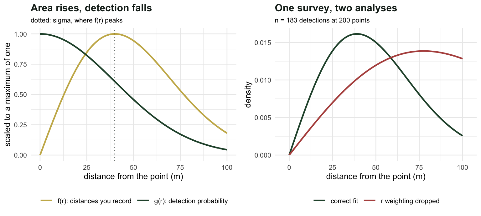
The same wrong model, two geometries
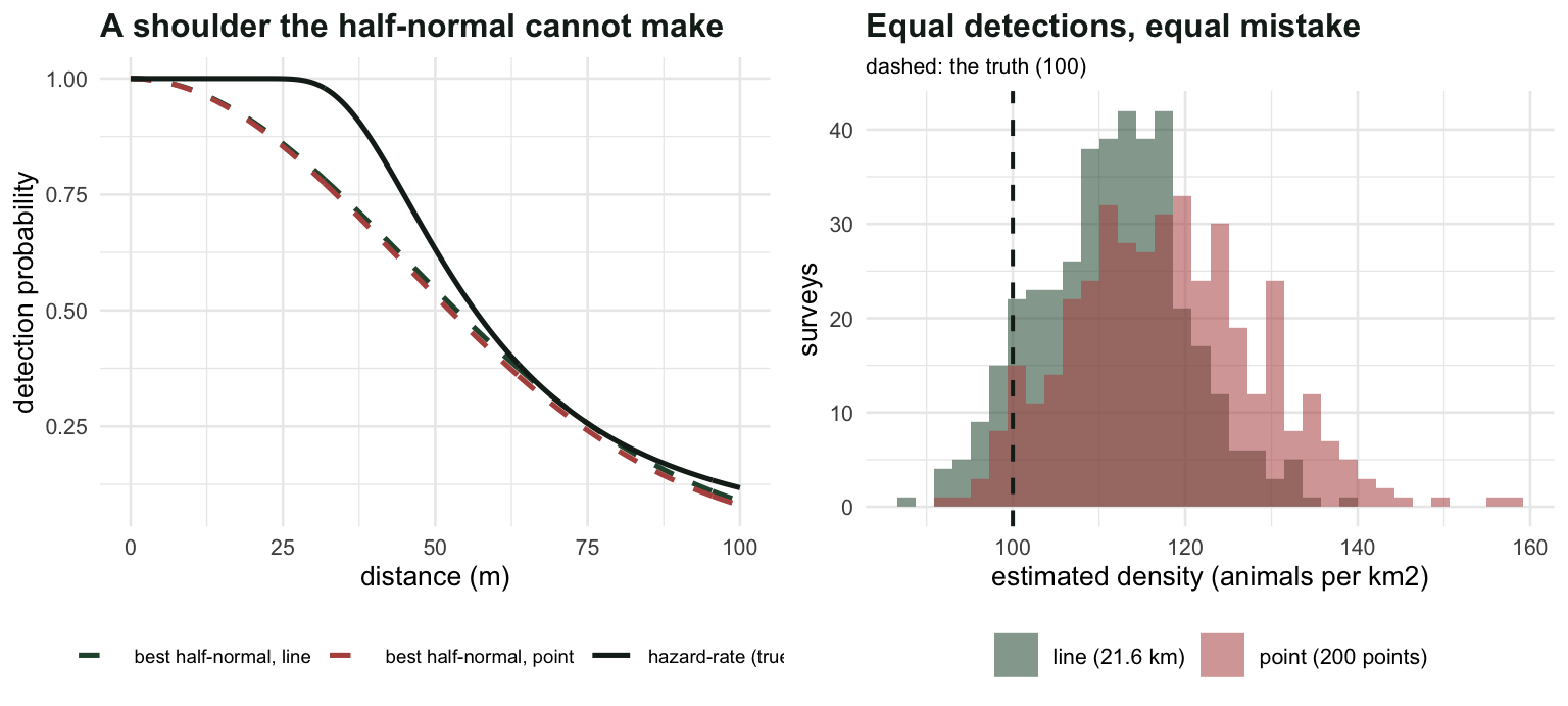
Now put the slope-versus-height claim to work. Take a world where the true detection function has a shoulder, which real detection functions usually do: everything close is seen, then detection falls away. A hazard-rate key produces that shape; a half-normal cannot. Fit the half-normal anyway, and compare what it costs on a line against what it costs at a point.
s_hr <- 0.05; b_hr <- 3
mu_t <- mu_hr(s_hr, b_hr, w); nu_t <- nu_hr(s_hr, b_hr, w)
sprintf("hazard-rate truth: g(0.5 sigma) = %.4f, g(sigma) = %.4f | mu %.5f | nu %.7f",
        g_hr(0.5*s_hr, s_hr, b_hr), g_hr(s_hr, s_hr, b_hr), mu_t, nu_t)
[1] "hazard-rate truth: g(0.5 sigma) = 0.9997, g(sigma) = 0.6321 | mu 0.06161 | nu 0.0021177"best_fit <- function(dens, ld, w) {
optimise(function(p) -integrate(function(x) dens(x)*ld(x, exp(p), w), 1e-9, w)$value,
c(-6, 0), tol = 1e-12)$minimum
}
sL <- exp(best_fit(function(x) g_hr(x, s_hr, b_hr)/mu_t, ld_ln, w))
sP <- exp(best_fit(function(r) r*g_hr(r, s_hr, b_hr)/nu_t, ld_pt, w))
sprintf("LINE : best half-normal sigma %.5f -> mu %.5f vs true %.5f -> D bias %+.2f%%",
sL, mu_hn(sL, w), mu_t, 100*(mu_t/mu_hn(sL, w) - 1))[1] "LINE : best half-normal sigma 0.04544 -> mu 0.05537 vs true 0.06161 -> D bias +11.27%"sprintf("POINT: best half-normal sigma %.5f -> nu %.7f vs true %.7f -> D bias %+.2f%%",
sP, nu_hn(sP, w), nu_t, 100*(nu_t/nu_hn(sP, w) - 1))[1] "POINT: best half-normal sigma 0.04445 -> nu 0.0018185 vs true 0.0021177 -> D bias +16.45%"The same key function, fitted to the same detection process, costs 11.3 per cent on a line and 16.5 per cent at a point: about 1.5 times worse. Both biases are positive, because a model with no shoulder fitted to shouldered data underestimates the effective width or radius, and dividing by too small an area inflates density.
The bias is not an approximation of anything. It is the error in that one number at the origin, restated: the ratio \(\hat{D}/D\) equals the ratio of fitted to true slope at zero, exactly, and the point geometry makes that slope harder to pin down.
Truncating harder is the usual reflex, and it does not rescue this.
sw <- t(sapply(c(0.06, 0.07, 0.08, 0.09, 0.10), function(ww) {
  nt <- nu_hr(s_hr, b_hr, ww); mt <- mu_hr(s_hr, b_hr, ww)
  sp <- exp(best_fit(function(r) r*g_hr(r, s_hr, b_hr)/nt, ld_pt, ww))
  sl <- exp(best_fit(function(x) g_hr(x, s_hr, b_hr)/mt, ld_ln, ww))
  c(w = ww, dropped_pct = 100*(1 - nt/nu_t),
    point_bias = 100*(nt/nu_hn(sp, ww) - 1), line_bias = 100*(mt/mu_hn(sl, ww) - 1))
}))
round(sw, 2)
w dropped_pct point_bias line_bias
[1,] 0.06 33.85 16.50 8.14
[2,] 0.07 22.61 20.00 10.45
[3,] 0.08 13.51 20.70 11.58
[4,] 0.09 6.10 19.27 11.77
[5,] 0.10 0.00 16.45 11.27Cutting the truncation radius back to 60 m throws away a third of the detections and leaves the point transect bias almost exactly where it started. The bias is not living in the tail.
Four hundred surveys of each
To compare the two designs fairly, give the line survey enough transect to expect the same number of detections as the 200 points, and let both analysts make the same modelling mistake.
Ln <- 266.1/(2*D*mu_t)
M <- 400
res <- t(sapply(1:M, function(i) {
  set.seed(52820 + i)
  Np <- rpois(1, D*K*pi*w^2); rp <- sqrt(runif(Np))*w
  rp <- rp[runif(Np) < g_hr(rp, s_hr, b_hr)]
  Nl <- rpois(1, D*2*w*Ln);   xl <- runif(Nl, 0, w)
  xl <- xl[runif(Nl) < g_hr(xl, s_hr, b_hr)]
  c(n_pt = length(rp), n_ln = length(xl),
    D_pt = length(rp)/(2*pi*K*nu_hn(fit_pt(rp, w), w)),
    D_ln = length(xl)/(2*Ln*mu_hn(fit_ln(xl, w), w)))
}))
sprintf("effort matched: %d points and %.1f km of line, both expecting %.0f detections",
        K, Ln, 2*D*Ln*mu_t)
[1] "effort matched: 200 points and 21.6 km of line, both expecting 266 detections"sprintf("POINT: D %.2f (SD %.2f) = %+.1f%% | within 5%% of the truth in %.1f%% of surveys",
mean(res[, "D_pt"]), sd(res[, "D_pt"]), 100*(mean(res[, "D_pt"])/D - 1),
100*mean(abs(res[, "D_pt"]/D - 1) < 0.05))[1] "POINT: D 117.81 (SD 10.83) = +17.8% | within 5% of the truth in 11.5% of surveys"sprintf("LINE : D %.2f (SD %.2f) = %+.1f%% | within 5%% of the truth in %.1f%% of surveys",
mean(res[, "D_ln"]), sd(res[, "D_ln"]), 100*(mean(res[, "D_ln"])/D - 1),
100*mean(abs(res[, "D_ln"]/D - 1) < 0.05))[1] "LINE : D 111.59 (SD 8.61) = +11.6% | within 5% of the truth in 21.8% of surveys"The simulated biases run a little above the exact asymptotic values (+16.5 and +11.3 per cent), which is what happens when you average a ratio: \(E[1/\hat{\nu}]\) sits above \(1/E[\hat{\nu}]\). The ordering is the point, and it is stable: equal detections, equal mistake, and the point survey lands near the truth half as often.
What this means in the field
The practical advice that falls out of the slope has been standard since Buckland (2006), and now it has a reason attached rather than a rule to memorise.
Prefer a key function with a shoulder, and be readier to add adjustment terms at a point than on a line. Group the distances rather than pretending 3 m of precision at 90 m, since binned data fitted with a multinomial likelihood are honest about what you measured. Record enough detections: the usual line transect target of 60 to 80 is thin for a point survey. And take the near-point measurements seriously, because that handful of birds inside half a sigma is carrying the slope.
What this does not fix
The estimator assumes the animals are uniformly distributed with respect to the point, which is a statement about where you put your points, not about the birds. Points placed at path junctions or in clearings break it, and no amount of care with the key function repairs a density gradient around the point.
It also assumes everything at the point is detected. On a line an observer walks along and can be reasonably sure of the animals on the line itself. Standing at a point, the birds directly overhead in the canopy are not obviously easier. That assumption is the subject of the checking post, and the short version is that your distances cannot test it.
Finally, this post held detection to a single key function with a single scale. Real point counts vary by observer, by time of morning, by wind and by species, all of which belong in the detection function rather than in the residual.
Distances estimated with error
Everything above takes the recorded distances as exact. Many point-count distances are judged: the observer hears a bird in the canopy and writes down 40 m. Rounding on line transects is the deterministic cousin, and digit preference the habit of favouring round numbers. Here the error is random and multiplicative, the kind Marques (2004) studied on line transects, and the recorded distance is \(r_o = r e^{\varepsilon}\) with \(\varepsilon\) normal with mean \(-s^2/2\) and standard deviation \(s\), right on average, with a coefficient of variation close to \(s\).
Without truncation there is a closed form. The error multiplies \(E[r^2]\) by \(e^{s^2}\), the untruncated half-normal fit sets \(\hat{\sigma}^2 = \overline{r^2}/2\), so \(\hat{\nu} = \hat{\sigma}^2\) is too large by \(e^{s^2}\) and the density too small by \(e^{-s^2}\). With truncation there is no simple formula, but where the naive fit converges is still a deterministic calculation: maximise the expected ld_pt under the distribution of recorded distances, the idea of best_fit above, on a grid (true distances out to 10 \(\sigma\), so errors carry birds across \(w\) in both directions; 100 normal quantiles for \(\varepsilon\)).
de_rg <- seq(5e-5, 0.4, by = 1e-4)                 # true distances, far beyond w
de_wr <- de_rg*g_hn(de_rg, s0); de_wr <- de_wr/sum(de_wr)
de_z  <- qnorm(ppoints(100))
de_asym <- function(se, ww, parts = FALSE) {       # limit of D-hat/D, naive fit
  ro <- outer(de_rg, exp(se*de_z - se^2/2))
  pw <- outer(de_wr, rep(1/length(de_z), length(de_z)))
  keep <- ro <= ww; p_in <- sum(pw[keep])
  s_star <- exp(optimise(function(q) -sum(pw[keep]*ld_pt(ro[keep], exp(q), ww)),
                         c(-6, 0), tol = 1e-12)$minimum)
  if (parts) return(c(p_in/(1 - g_hn(ww, s0)), nu_hn(s_star, ww)/nu_hn(s0, ww),
                      sum(pw[keep]*ro[keep]^2)/p_in/m2_point(s0, ww)))
  p_in*s0^2/nu_hn(s_star, ww)
}
de_s <- c(0.1, 0.2, 0.3, 0.4); de_w <- c(2, 2.5, 3, 3.5, 4, 8)
de_tab <- sapply(de_s, function(se) sapply(de_w*s0, function(ww) de_asym(se, ww)))
dimnames(de_tab) <- list(paste(de_w, "sigma"), paste("s =", de_s))
stopifnot(abs(de_asym(0, w) - 1) < 1e-3, abs(de_tab["8 sigma", 1:3] - exp(-de_s[1:3]^2)) < 0.01)
round(rbind(de_tab, "no truncation, exp(-s^2)" = exp(-de_s^2)), 3)
s = 0.1 s = 0.2 s = 0.3 s = 0.4
2 sigma 1.021 1.080 1.172 1.289
2.5 sigma 1.013 1.049 1.105 1.178
3 sigma 1.004 1.019 1.046 1.088
3.5 sigma 0.997 0.995 1.000 1.018
4 sigma 0.993 0.979 0.967 0.967
8 sigma 0.990 0.962 0.917 0.861
no truncation, exp(-s^2) 0.990 0.961 0.914 0.852de_parts <- de_asym(0.3, w, parts = TRUE)
sprintf("w = 2.5 sigma, s = 0.3: share inside w %.3f of error-free | mean r^2 inside w %.3f of error-free | fitted nu %.3f of true",
de_parts[1], de_parts[3], de_parts[2])[1] "w = 2.5 sigma, s = 0.3: share inside w 0.970 of error-free | mean r^2 inside w 0.907 of error-free | fitted nu 0.878 of true"At this survey’s truncation, 2.5 \(\sigma\), the naive fit converges to 1.049 of the true density at \(s\) = 0.2 and 1.105 at \(s\) = 0.3; at 2 \(\sigma\) the same errors give 1.080 and 1.172. The sign turns between 3 and 4 \(\sigma\), near 3.5 \(\sigma\) with the exact point depending on \(s\), and the untruncated \(e^{-s^2}\) is approached at 8 \(\sigma\) (within 0.01 for \(s \le 0.3\), checked in the chunk). The truncation turns the bias around. The errors scatter distances both ways: the scatter towards the point stays in the data, while the scatter out past \(w\) is cut off (at \(s\) = 0.3 the share inside \(w\) falls to 0.970 of its error-free value). The distances that remain sit closer to the point than the truth, with a mean square 0.907 of the error-free one, so the half-normal reads a smaller scale. The fitted \(\nu\) drops to 0.878 of the true one, further than the count, and the density comes out high. The truncation radius, chosen for other reasons, sets the sign.
Marques (2004) corrects line-transect estimates when the error distribution is known. At a point, one way to do it is a likelihood that integrates over the error. A recorded distance inside \(w\) has density proportional to \(\int x\,g(x)\,\mathrm{LN}(r_o \mid \log x - s^2/2, s)\,\mathrm{d}x\), normalised by \(P_w = \int x\,g(x)\,P(r_o \le w \mid x)\,\mathrm{d}x\), and \(\hat{D} = n/(2\pi K P_w)\). It needs \(s\): once as known, once estimated from 30 birds whose distance was judged twice (the standard deviation of the log ratio of the two readings over \(\sqrt{2}\)). Each simulated survey also gets the fit to the true distances, which carries the small-sample excess of \(E[1/\hat{\nu}]\) seen in the four hundred surveys above.
de_xg <- seq(1e-4, 0.25, by = 5e-4)                # grid of true distances for the fix
de_fit_err <- function(o, se) {
  kern <- outer(o, de_xg, function(a, x) dlnorm(a, log(x) - se^2/2, se))
  p_w  <- plnorm(w, log(de_xg) - se^2/2, se)       # P(recorded <= w | true x)
  nll  <- function(q) { gx <- de_xg*g_hn(de_xg, exp(q))
    -sum(log(kern %*% gx)) + length(o)*log(sum(p_w*gx)) }
  sg <- exp(optimise(nll, c(-6, -1), tol = 1e-8)$minimum)
  length(o)/(2*pi*K*sum(p_w*de_xg*g_hn(de_xg, sg))*5e-4)
}
set.seed(34510); de_M <- 1000
de_mc <- t(replicate(de_M, {
  n_all <- rpois(1, D*K*pi*0.25^2); r_true <- sqrt(runif(n_all))*0.25
  r_true <- r_true[runif(n_all) < g_hn(r_true, s0)]
  z_err <- rnorm(length(r_true)); z_rep <- rnorm(30) - rnorm(30)
  out <- c(exact = sum(r_true <= w)/(2*pi*K*nu_hn(fit_pt(r_true[r_true <= w], w), w)))
  for (se in c(0.2, 0.3)) {
    o <- r_true*exp(se*z_err - se^2/2); o <- o[o <= w]
    out <- c(out, setNames(c(length(o)/(2*pi*K*nu_hn(fit_pt(o, w), w)), de_fit_err(o, se),
                             de_fit_err(o, se*sd(z_rep)/sqrt(2))), paste0(c("naive", "known", "est"), se)))
  }
  out
}))/D
de_mean <- colMeans(de_mc); de_sd <- apply(de_mc, 2, sd)
de_pair <- de_mc[, c("naive0.2", "naive0.3")] - de_mc[, "exact"]
sprintf("%s: mean D/D %.3f (MC SE %.3f), survey SD %.3f", names(de_mean), de_mean, de_sd/sqrt(de_M), de_sd)
[1] "exact: mean D/D 1.009 (MC SE 0.004), survey SD 0.113"
[2] "naive0.2: mean D/D 1.062 (MC SE 0.004), survey SD 0.121"
[3] "known0.2: mean D/D 1.012 (MC SE 0.004), survey SD 0.122"
[4] "est0.2: mean D/D 1.011 (MC SE 0.004), survey SD 0.123"
[5] "naive0.3: mean D/D 1.118 (MC SE 0.004), survey SD 0.129"
[6] "known0.3: mean D/D 1.012 (MC SE 0.004), survey SD 0.130"
[7] "est0.3: mean D/D 1.010 (MC SE 0.004), survey SD 0.136" sprintf("naive minus exact, same birds: s = %.1f %+.3f (MC SE %.3f) | limit %+.3f",
c(0.2, 0.3), colMeans(de_pair), apply(de_pair, 2, sd)/sqrt(de_M), de_tab["2.5 sigma", 2:3] - 1)[1] "naive minus exact, same birds: s = 0.2 +0.053 (MC SE 0.002) | limit +0.049"
[2] "naive minus exact, same birds: s = 0.3 +0.109 (MC SE 0.002) | limit +0.105"In a thousand surveys of this design the fit to the true distances averages 1.009 of the truth (MC SE 0.004), a little above one as the small-sample excess predicts, and the naive fit 1.062 at \(s\) = 0.2 and 1.118 at \(s\) = 0.3. On the same birds the naive fit runs +0.053 and +0.109 above the exact one, against limits of +0.049 and +0.105: a gap of at most 0.004, about 2 Monte Carlo standard errors, small beside the bias. The error-aware fit, with \(s\) known or estimated from the 30 repeat pairs, averages within 0.004 of the fit to the true distances. It removes the bias, not the information the errors destroyed: the survey-to-survey SD is 0.113 with true distances and 0.130 with the fix at \(s\) = 0.3, and estimating \(s\) from 30 pairs raises it to 0.136, in this design.
All of this assumes mean-preserving lognormal error with one \(s\) for every bird. An observer who underestimates far birds makes the same mistake on both readings, and the repeat pairs cannot see it. Whether grouping the distances into intervals, as advised above, changes the bias was not tested here. The repeat measurement of a subset that the checking post lists under accurate distances is the input this fit needs.
Adding plain point counts
Many monitoring schemes hold far more plain point counts than distance data: the observer stood at the point, counted the birds and wrote down no distances. Kery et al. (2024) treat such counts as distance surveys whose distances went unrecorded and fit both kinds of data in one integrated distance sampling model.
Keep the survey above (200 points, \(\sigma\) = 40 m, truncation at 100 m) and add 800 points where the observer counts every bird within the same 100 m and records no distance. If detection is the same under both protocols, the joint fit separates cleanly. The scale comes from the distances alone (fit_pt, as before), every point has the same expected count \(2\pi D\nu\), and \(\hat{D}\) is the total count from both protocols divided by \(2\pi (K_d + K_p)\hat{\nu}\). With Poisson counts its variance has two terms:
\[\mathrm{Var}(\log\hat{D}) \approx \frac{1}{(K_d + K_p)\,\mu} + \frac{c}{K_d\,\mu}, \qquad c = \frac{(\mathrm{d}\log\nu/\mathrm{d}\log\sigma)^2}{\mathrm{Var}_f(r^2/\sigma^2)}\]
with \(\mu\) the expected number of detections per point. The first term is the encounter rate, and every point shrinks it. The second is the uncertainty in \(\hat{\nu}\): the denominator of \(c\) is the information one detection carries about \(\log\sigma\), and only the distance points supply it. Without truncation \(\nu = \sigma^2\) and \(r^2/\sigma^2\) is exponential with mean 2, so \(c = 4/4 = 1\). Truncation at 2.5 \(\sigma\) makes it larger.
pc_Kd <- K; pc_Kp <- 4*K; pc_rho <- 0.8          # 200 distance points, 800 plain counts
pc_mu <- D*2*pi*nu0                               # expected detections per point
pc_dl <- function(s, wr) { a <- wr^2/(2*s^2); if (is.finite(a)) 2 - 2*a*exp(-a)/(1 - exp(-a)) else 2 }
pc_dlnu <- pc_dl(s0, w)                           # d log nu / d log sigma
stopifnot(abs(pc_dlnu - log(nu_hn(s0*1.001, w)/nu_hn(s0/1.001, w))/(2*log(1.001))) < 1e-5)
pc_mom <- function(k) integrate(function(x) (x^2/s0^2)^k*fpt(x, s0, w), 0, w)$value
pc_I  <- pc_mom(2) - pc_mom(1)^2                  # information per detection on log sigma
pc_c  <- pc_dlnu^2/pc_I
pc_se <- function(Kd, Kp) sqrt(1/((Kd + Kp)*pc_mu) + pc_c/(Kd*pc_mu))
pc_r  <- nu_hn(pc_rho*s0, w)/nu0                  # plain counts with sigma_p = 0.8 sigma
pc_lim <- (pc_Kd + pc_Kp*pc_r)/(pc_Kd + pc_Kp)
sprintf("mu %.4f per point | c %.4f | detection term %.1f%% of the distance-only variance",
        pc_mu, pc_c, 100*pc_c/(1 + pc_c))
[1] "mu 0.9611 per point | c 1.3822 | detection term 58.0% of the distance-only variance"sprintf("SE of log D: distances only %.4f | with %d plain counts %.4f (%+.1f%%) | floor %.4f (%+.1f%%)",
pc_se(pc_Kd, 0), pc_Kp, pc_se(pc_Kd, pc_Kp), 100*(pc_se(pc_Kd, pc_Kp)/pc_se(pc_Kd, 0) - 1),
sqrt(pc_c/(pc_Kd*pc_mu)), 100*(sqrt(pc_c/(1 + pc_c)) - 1))[1] "SE of log D: distances only 0.1113 | with 800 plain counts 0.0907 (-18.5%) | floor 0.0848 (-23.8%)"sprintf("sigma_p = %.1f sigma: r = %.4f (rho^2 = %.2f) | shared fit converges to %.4f D",
pc_rho, pc_r, pc_rho^2, pc_lim)[1] "sigma_p = 0.8 sigma: r = 0.6643 (rho^2 = 0.64) | shared fit converges to 0.7315 D"Eight hundred plain counts take the standard error of \(\log\hat{D}\) from 0.111 to 0.091, 18.5 per cent less, and no number of them can take it more than 24 per cent below the distance-only value, because the detection term is 58 per cent of the distance-only variance and plain counts never touch it.
That assumes the two protocols share a detection function. Suppose instead that the plain counts see less far, \(\sigma_p = 0.8\sigma\). A shared fit then converges to \(D (K_d + K_p r)/(K_d + K_p)\) with \(r = \nu(0.8\sigma, w)/\nu(\sigma, w)\) = 0.664, not \(0.8^2\) = 0.64: truncation removes a larger share of the distance observer’s detections than of the plain counter’s. The simulation below reproduces both closed forms and adds a second world, where the plain counts detect as well as the distance observer but sit in habitat with fewer birds, \(D r\) per km2.
pc_draw <- function(npt, sig, dens) {             # counts and distances within w
  n_in <- rpois(npt, dens*pi*w^2)
  rr <- sqrt(runif(sum(n_in)))*w
  seen <- runif(length(rr)) < g_hn(rr, sig)
  list(n = tabulate(rep.int(seq_len(npt), n_in)[seen], npt), r = rr[seen])
}
## shared against separate sigma for the plain counts: the distances enter both fits alike
pc_ll  <- function(y) sum(dpois(y, mean(y), log = TRUE))
pc_lrt <- function(a, b) 2*(pc_ll(a) + pc_ll(b) - pc_ll(c(a, b)))
pc_one <- function() {
  dd <- pc_draw(pc_Kd, s0, D); nuh <- nu_hn(fit_pt(dd$r, w), w)
  p_same <- pc_draw(pc_Kp, s0, D)$n
  p_det  <- pc_draw(pc_Kp, pc_rho*s0, D)$n        # plain counts see less far
  p_hab  <- pc_draw(pc_Kp, s0, D*pc_r)$n          # plain-count points hold fewer birds
  shared <- function(p) sum(dd$n, p)/(2*pi*(pc_Kd + pc_Kp)*nuh)
  se_sh  <- sqrt(1/sum(dd$n, p_det) + pc_c/length(dd$r))
  c(D_ds = sum(dd$n)/(2*pi*pc_Kd*nuh), D_same = shared(p_same), D_det = shared(p_det),
    cov_det = abs(log(shared(p_det)/D)) < 1.96*se_sh,
    lrt_same = pc_lrt(dd$n, p_same), lrt_det = pc_lrt(dd$n, p_det), lrt_hab = pc_lrt(dd$n, p_hab),
    Dp_hab = mean(p_hab)/(2*pi*nuh))
}
set.seed(34120)
pc_R <- 2000
pc_sim <- t(replicate(pc_R, pc_one()))
pc_rej <- colMeans(pc_sim[, c("lrt_same", "lrt_det", "lrt_hab")] > qchisq(0.95, 1))
sprintf("SD of log D: distances only %.4f | with plain counts %.4f (MC SE %.4f)",
        sd(log(pc_sim[, "D_ds"])), sd(log(pc_sim[, "D_same"])),
        sd(log(pc_sim[, "D_same"]))/sqrt(2*(pc_R - 1)))
[1] "SD of log D: distances only 0.1114 | with plain counts 0.0902 (MC SE 0.0014)"pc_mcse <- apply(pc_sim[, c("D_ds", "D_same", "D_det")]/D, 2, sd)/sqrt(pc_R)
sprintf("mean D/D (MC SE): distances only %.4f (%.4f) | shared, same detection %.4f (%.4f) | shared, sigma_p 0.8 %.4f (%.4f)",
mean(pc_sim[, "D_ds"])/D, pc_mcse[1], mean(pc_sim[, "D_same"])/D, pc_mcse[2],
mean(pc_sim[, "D_det"])/D, pc_mcse[3])[1] "mean D/D (MC SE): distances only 1.0017 (0.0025) | shared, same detection 1.0003 (0.0020) | shared, sigma_p 0.8 0.7322 (0.0015)"## E[nu/nu-hat] - 1 to second order in log sigma-hat, its small-sample bias included
pc_L <- function(h) log(nu_hn(s0*exp(h), w))
pc_L2 <- (pc_L(1e-3) - 2*pc_L(0) + pc_L(-1e-3))/1e-6
pc_L3 <- (pc_L(2e-3) - 2*pc_L(1e-3) + 2*pc_L(-1e-3) - pc_L(-2e-3))/2e-9
pc_b <- (4*pc_mom(1) - pc_L3 - 4*pc_I)/(2*pc_Kd*pc_mu*pc_I^2)
pc_exc <- -pc_dlnu*pc_b - (pc_L2 - pc_dlnu^2)/(2*pc_Kd*pc_mu*pc_I)
pc_dev <- (colMeans(pc_sim[, c("D_ds", "D_same", "D_det")])/D - c(1, 1, pc_lim)*(1 + pc_exc))/pc_mcse
stopifnot(all(abs(pc_dev) < 2))
sprintf("small-sample excess %.2f%% | mean minus raised limit, in MC SE: %s", 100*pc_exc, toString(sprintf("%+.2f", pc_dev)))[1] "small-sample excess 0.41% | mean minus raised limit, in MC SE: -0.98, -1.89, -1.53"sprintf("sigma_p 0.8: 95%% interval covers D in %.3f | LRT rejects: same %.3f, sigma_p %.3f, habitat %.3f",
mean(pc_sim[, "cov_det"]), pc_rej[1], pc_rej[2], pc_rej[3])[1] "sigma_p 0.8: 95% interval covers D in 0.073 | LRT rejects: same 0.059, sigma_p 0.994, habitat 0.992"sprintf("habitat world, shared sigma with its own D at the plain-count points: %.2f", mean(pc_sim[, "Dp_hab"]))[1] "habitat world, shared sigma with its own D at the plain-count points: 66.53"## what the plain counts still inform: a habitat slope, log D = log(100) + 0.3 x
set.seed(34121)
pc_b1 <- 0.3
pc_slope <- function() {
xd <- rnorm(pc_Kd); xp <- rnorm(pc_Kp)
nd <- pc_draw(pc_Kd, s0, D*exp(pc_b1*xd))$n; np <- pc_draw(pc_Kp, s0, D*exp(pc_b1*xp))$n
one <- glm.fit(cbind(1, xd), nd, family = poisson()) # nu only shifts the intercept
two <- glm.fit(cbind(rep(1:0, c(pc_Kd, pc_Kp)), rep(0:1, c(pc_Kd, pc_Kp)), c(xd, xp)),
c(nd, np), family = poisson()) # own intercept for the plain counts
c(ds = one$coefficients[[2]], joint = two$coefficients[[3]])
}
pc_sl <- t(replicate(500, pc_slope()))
sprintf("slope (true %.1f): distances only %.3f (SD %.4f) | with plain counts %.3f (SD %.4f)",
pc_b1, mean(pc_sl[, "ds"]), sd(pc_sl[, "ds"]), mean(pc_sl[, "joint"]), sd(pc_sl[, "joint"]))[1] "slope (true 0.3): distances only 0.304 (SD 0.0783) | with plain counts 0.300 (SD 0.0326)"pc_slse <- 1/sqrt(c(pc_Kd, pc_Kd + pc_Kp)*pc_mu*exp(pc_b1^2/2)) # large-sample SD of the slope
sprintf("large-sample SD of the slope: distances only %.4f | with plain counts %.4f", pc_slse[1], pc_slse[2])[1] "large-sample SD of the slope: distances only 0.0705 | with plain counts 0.0315"With a shared detection function the simulated standard deviation of \(\log\hat{D}\) falls from 0.111 to 0.090, which reproduces the closed form by simulation. When the plain counts see less far, the shared fit averages 0.732 of the true density against the limit of 0.731, and its 95 per cent interval covers the truth in 7 per cent of surveys. The simulated means should sit slightly above their limits, by the small-sample excess of \(E[1/\hat{\nu}]\) over \(1/\nu\) seen in the four hundred surveys; to second order in \(\log\hat{\sigma}\) it is 0.4 per cent for 200 points, and all three means lie within two Monte Carlo standard errors of their limits raised by that much.
In a survey this size, a mismatch this large does not go unnoticed. The likelihood ratio test of a shared against a separate detection scale for the plain counts rejects in 99.4 per cent of surveys, and at a rate of 0.059 (nominal 0.05) when nothing differs. The integrated models of Kery et al. (2024) allow each data type its own detection function, the obvious response, but it has a price. With a constant density, a free \(\sigma_p\) makes the plain-count mean a free parameter, so \(\hat{D}\) is the distance-only estimate exactly, and the 800 counts add nothing on density beyond the bound that detection cannot exceed one. What they still inform is anything the two protocols share beyond an intercept. For a habitat slope \(b\) = 0.3 on a standard normal covariate, every point carries the same information on the slope whichever protocol it uses, so its large-sample standard deviation, \(1/\sqrt{K\mu e^{b^2/2}}\) over the \(K\) points, falls from 0.071 to 0.032. The 500 simulated surveys give 0.078 and 0.033, the distance-only value on the high side of its Monte Carlo spread. The split between intercept and slope is the same arithmetic as in hierarchical distance sampling, where a detection bias that is constant across sites moves the intercept and leaves the slope alone.
The test also cannot say what it has found. The likelihood sees the plain counts only through their mean, \(2\pi D_p\,\nu(\sigma_p, w)\), so poorer detection and fewer birds give exactly the same distribution of counts. In the habitat world the test rejects in 99.2 per cent of surveys, as it did in the detection world. A model with a separate \(\sigma_p\) puts the plain-count points at the distance-only density, near 100; a model with a shared \(\sigma\) and its own density there puts them at 66.5. Both fit equally well: each reproduces the mean count of both protocols exactly. The first is right when the plain counts see less far, and the second when the habitat is poorer, so the two defensible fixes move the plain-count density in opposite directions from the shared fit’s 73. The source-conflict check in checking an integrated SDM finds a disagreement of this kind; there the survey is unbiased by design, so a failed check says which source to distrust. Here nothing in the data says it. The remedy is design: assign the protocols to points at random, so habitat can differ between them only by chance, or run both protocols at some calibration points.
## plain counts without a radius: the count now depends on the tail beyond w
pc_nu <- function(s, wr) if (is.finite(wr)) nu_hn(s, wr) else s^2
pc_info <- function(wp) {                          # expected information, (log D, log sigma)
  gd <- c(1, pc_dl(s0, w)); gp <- c(1, pc_dl(s0, wp))
  pc_Kd*pc_mu*gd %o% gd + pc_Kp*D*2*pi*pc_nu(s0, wp)*gp %o% gp +
    diag(c(0, pc_Kd*pc_mu*pc_I))
}
pc_sdw <- sapply(c(w, Inf), function(wp) sqrt(solve(pc_info(wp))[1, 1]))
stopifnot(all.equal(pc_sdw[1], pc_se(pc_Kd, pc_Kp)))
pc_pseudo <- function(wp) {                        # where the shared fit converges, sigma_p = 0.8 sigma
  mp <- D*2*pi*pc_nu(pc_rho*s0, wp)
  nll <- function(p) {
    ld <- exp(p[1])*2*pi*nu_hn(exp(p[2]), w); lp <- exp(p[1])*2*pi*pc_nu(exp(p[2]), wp)
    -(pc_Kd*(pc_mu*log(ld) - ld) + pc_Kp*(mp*log(lp) - lp) +
      pc_Kd*pc_mu*(-pc_mom(1)*s0^2/(2*exp(2*p[2])) - log(nu_hn(exp(p[2]), w))))
  }
  exp(optim(c(log(D), log(s0)), nll, method = "BFGS", control = list(reltol = 1e-14))$par)/c(D, s0)
}
pc_ps <- sapply(c(w, Inf), pc_pseudo)
sprintf("plain counts within w: SE %.4f, shared fit D/D %.4f, sigma/sigma %.4f", pc_sdw[1], pc_ps[1, 1], pc_ps[2, 1])
[1] "plain counts within w: SE 0.0907, shared fit D/D 0.7315, sigma/sigma 1.0000"sprintf("plain counts, no radius: SE %.4f, shared fit D/D %.4f, sigma/sigma %.4f", pc_sdw[2], pc_ps[1, 2], pc_ps[2, 2])[1] "plain counts, no radius: SE 0.1000, shared fit D/D 0.7538, sigma/sigma 0.9693"Last, the plain counts need the truncation radius of the distance protocol. Without it the count depends on the half-normal tail beyond \(w\), which the truncation was chosen to keep out of the analysis. The standard error is then 0.100 rather than 0.091, and when the plain counts see less far the shared fit no longer leaves the distances alone: it pulls \(\hat{\sigma}\) to 0.969 of the truth, while the density bias changes little (0.754 of the truth against 0.731).
References
Buckland ST 2006 The Auk 123(2):345-357 (10.1093/auk/123.2.345)
Buckland ST, Rexstad EA, Marques TA, Oedekoven CS 2015 Distance Sampling: Methods and Applications, Springer, ISBN 978-3-319-19218-5
Kery M, Royle JA, Hallman TA, Robinson WD, Strebel N, Kellner KF 2024 Ecology 105(5):e4292 (10.1002/ecy.4292)
Marques FFC, Buckland ST 2003 Biometrics 59(4):924-935 (10.1111/j.0006-341X.2003.00107.x)
Marques TA 2004 Biometrics 60(3):757-763 (10.1111/j.0006-341X.2004.00226.x)
Marques TA, Thomas L, Fancy SG, Buckland ST 2007 The Auk 124(4):1229-1243 (10.1093/auk/124.4.1229)
Rexstad E, Buckland ST, Marshall L, Borchers D 2023 Ecology and Evolution 13(1):e9684 (10.1002/ece3.9684)