---
title: "Density surface models for distance sampling"
description: "Two-stage density surface modelling in R: fitting a detection function, a spatial GAM on segments, and the variance term the naive interval leaves out."
date: "2026-06-17 14:00"
date-modified: "2026-10-14"
categories: [R, distance sampling, abundance, imperfect detection, ecology tutorial]
image: thumbnail.png
image-alt: "A bar chart of the coverage of a nominal 95% interval across 300 simulated line transect surveys. The bar for spatial variance only reaches 83.3 per cent and the bar for detection variance added reaches 92.3 per cent, both under a dashed line drawn at the nominal 95 per cent."
---
*Corrected 14 October 2026: the heading and the close of the section on the propagated interval still treated its shortfall from nominal coverage as real, asking why it falls short and calling the propagation most of the available repair; they now ask how close it comes and say the propagation may be all the repair this simulation needs. The spatial-only coverage is now given as a result of these replicates rather than as the coverage itself, and a code comment now says that predict ignores an offset passed to gam as an argument.*
*Corrected 7 October 2026: the coverage section said that a survey reported as plus or minus eight per cent is really plus or minus twelve, treating the spread across the simulated surveys, itself a Monte Carlo estimate, as the true precision; it now gives a range running from the propagated figure to that spread.*
*Corrected 1 October 2026: the section on why the propagated interval is still not at its nominal coverage treated the remaining shortfall as real and named two causes for it; it now gives the Monte Carlo standard error of that coverage, says the rest of the gap may be simulation noise, and presents the two omissions as unmeasured here.*
[Line transect distance sampling](../distance-sampling-line-transect/) gives you one number: density, averaged over the survey region. That is often not the question. If you want to know where the animals are, or to predict abundance in a block nobody surveyed, you need the density to vary in space, and you need a model for how.
Density surface modelling is the standard answer, and its structure is worth understanding before its code. It has two stages, and the join between them is where the interesting failure lives.
## The two stages
Stage one fits a detection function to the perpendicular distances, exactly as in ordinary distance sampling. This gives you the effective strip half-width: the width of a hypothetical strip in which you would have detected everything, which is what turns a count into a density.
Stage two chops the transect lines into segments, counts detections per segment, and fits a spatial model to those counts with the effective area of the segment as an offset. Predict over a grid, sum, and you have abundance.
The join is that stage two takes stage one's answer as if it were a fact. It is not; it is an estimate with a standard error, and pretending otherwise is the thing this post measures.
## Setup
A region thirty by twenty kilometres. True density has a smooth peak, plus a floor everywhere. Ten transect lines. Half-normal detection with a truncation distance of 250 metres.
```{r data}
set.seed(3130)
suppressPackageStartupMessages(library(mgcv))

W <- 0.25                                        # truncation distance, km
dens_fun <- function(x, y) 8 * exp(-((x - 9)^2 / 60 + (y - 13)^2 / 30)) + 1.2
lines_x <- seq(1.5, 28.5, by = 3)
esw_of <- function(s) s * sqrt(pi / 2) * (2 * pnorm(W / s) - 1)

sim_survey <- function(sigma, seed) {
  set.seed(seed)
  lam_max <- dens_fun(9, 13)
  n0 <- rpois(1, lam_max * 30 * 20)
  px <- runif(n0, 0, 30); py <- runif(n0, 0, 20)
  keep <- runif(n0) < dens_fun(px, py) / lam_max     # thin to the true surface
  px <- px[keep]; py <- py[keep]
  obs <- do.call(rbind, lapply(lines_x, function(lx) {
    d <- abs(px - lx); cand <- which(d <= W)
    if (!length(cand)) return(NULL)
    seen <- cand[runif(length(cand)) < exp(-d[cand]^2 / (2 * sigma^2))]
    if (!length(seen)) return(NULL)
    data.frame(line = lx, dist = d[seen], y = py[seen])
  }))
  list(obs = obs, N_true = length(px))
}
sv <- sim_survey(sigma = 0.10, seed = 11)
p313_Ntrue <- sv$N_true; p313_ndet <- nrow(sv$obs)
c(true_N = p313_Ntrue, detections = p313_ndet)
```
## Stage one: the detection function
```{r detfun}
nll_hn <- function(lsig, d) {
  s <- exp(lsig)
  sum(d^2) / (2 * s^2) + length(d) * log(esw_of(s))
}
f1 <- optim(log(0.1), nll_hn, d = sv$obs$dist, method = "BFGS", hessian = TRUE)
sig_hat <- exp(f1$par)
esw <- esw_of(sig_hat)
p_hat <- esw / W                                  # average detection probability
se_sig <- sig_hat * sqrt(1 / f1$hessian[1, 1])
grad <- (esw_of(sig_hat * 1.001) - esw_of(sig_hat * 0.999)) / (0.002 * sig_hat)
se_p <- abs(grad) * se_sig / W                    # delta method

p313_sig <- sig_hat; p313_esw <- esw; p313_p <- p_hat
p313_sep <- se_p; p313_cvp <- se_p / p_hat
c(sigma = sig_hat, esw_km = esw, p = p_hat, se_p = se_p, cv_p = p313_cvp)
```
Sigma comes out at `r sprintf("%.4f", p313_sig)` against a true 0.10. The effective strip half-width is `r sprintf("%.0f", 1000 * p313_esw)` metres, so on average we detected `r sprintf("%.1f%%", 100 * p313_p)` of the animals inside the truncation distance. That estimate has a coefficient of variation of `r sprintf("%.1f%%", 100 * p313_cvp)`, which sounds small. Hold that thought.
## Stage two: the spatial model
Segments are two kilometres of line. Each one gets a count and an effective area of twice the half-width times the length.
```{r segments}
segs <- expand.grid(line = lines_x, y0 = seq(0, 18, by = 2))
segs$ymid <- segs$y0 + 1
segs$n <- mapply(function(lx, y0)
  sum(sv$obs$line == lx & sv$obs$y >= y0 & sv$obs$y < y0 + 2), segs$line, segs$y0)
segs$area <- 2 * esw * 2                          # effective area, km^2

m <- gam(n ~ s(line, ymid, k = 20), offset = log(area), family = poisson,
         data = segs, method = "REML")
p313_edf <- sum(m$edf); p313_dev <- summary(m)$dev.expl
p313_nseg <- nrow(segs); p313_nonzero <- sum(segs$n > 0)
c(segments = p313_nseg, with_detections = p313_nonzero,
  edf = p313_edf, deviance_explained = p313_dev)
```
The offset is doing the real work. It says: this segment had this much effective search area, so a count of three here means something different from a count of three on a segment half as long, or a segment surveyed when detection was poorer. Everything the detection function knows enters the spatial model through that one term. That is worth saying twice, because it is why stage one's error propagates the way it does: the offset is a *multiplier* on the whole surface, not a nuisance on one segment.
```{r predict}
grid <- expand.grid(line = seq(0.5, 29.5, 1), ymid = seq(0.5, 19.5, 1))
grid$area <- 1           # predict() ignores gam()'s offset argument: exp(lp) is per km^2
lp <- predict(m, newdata = grid, type = "link")
N_hat <- sum(exp(lp))
p313_N <- N_hat
c(N_hat = N_hat, true = p313_Ntrue, ratio = N_hat / p313_Ntrue)
```
```{r fig-surface}
#| echo: false
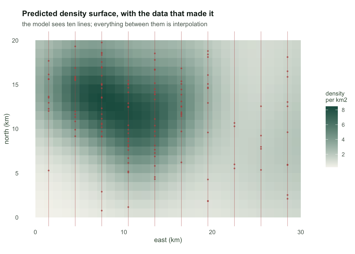
#| fig-cap: "Predicted density surface with the transect lines overlaid. Detections are shown as points on the lines; the surface between lines is the model's guess."
#| fig-alt: "Heatmap of predicted density across a thirty by twenty kilometre region, in a pale to dark green gradient with a broad high-density region in the left centre. Ten vertical transect lines are drawn in rust, with detection points scattered along them, densest where the surface is darkest."
library(ggplot2)
theme_te <- function() {
theme_minimal(base_size = 11) +
theme(
plot.background = element_rect(fill = "#f5f4ee", colour = NA),
panel.background = element_rect(fill = "#f5f4ee", colour = NA),
panel.grid = element_blank(),
plot.title = element_text(colour = "#16241d", face = "bold", size = 11),
plot.subtitle = element_text(colour = "#5d6b61", size = 9),
axis.title = element_text(colour = "#46604a", size = 9.5),
axis.text = element_text(colour = "#5d6b61", size = 8.5),
legend.title = element_text(colour = "#46604a", size = 8.5),
legend.text = element_text(colour = "#5d6b61", size = 8))
}
gp <- grid; gp$dens <- exp(lp)
ggplot(gp, aes(line, ymid)) +
geom_raster(aes(fill = dens)) +
geom_vline(xintercept = lines_x, colour = "#b5534e", linewidth = 0.25, alpha = 0.6) +
geom_point(data = sv$obs, aes(line, y), colour = "#b5534e", size = 0.5, alpha = 0.7) +
scale_fill_gradient(low = "#f5f4ee", high = "#1d5b4e", name = "density\nper km2") +
coord_fixed() +
labs(title = "Predicted density surface, with the data that made it",
subtitle = "the model sees ten lines; everything between them is interpolation",
x = "east (km)", y = "north (km)") +
theme_te()
```
Estimated abundance is `r sprintf("%.0f", p313_N)` against a true `r p313_Ntrue`. Close enough that you would believe it, which is the setup for the actual point.
## The variance that goes missing
The GAM has a standard error. Sum the predictions and propagate through the model coefficients, and you get a variance for the total. It is easy, it is what the software gives you, and it is not the answer.
```{r variance}
X <- predict(m, newdata = grid, type = "lpmatrix")
mu <- exp(lp)
dN_dbeta <- as.numeric(t(mu) %*% X)
var_spatial <- as.numeric(t(dN_dbeta) %*% vcov(m) %*% dN_dbeta)

# abundance scales as 1/p, so dN/dp = -N/p
var_detect <- (N_hat / p_hat)^2 * se_p^2

p313_vsp <- var_spatial; p313_vdet <- var_detect
p313_cv_naive <- sqrt(var_spatial) / N_hat
p313_cv_prop <- sqrt(var_spatial + var_detect) / N_hat
p313_share <- var_detect / (var_spatial + var_detect)
c(cv_spatial_only = p313_cv_naive, cv_propagated = p313_cv_prop,
  detection_share = p313_share)
```
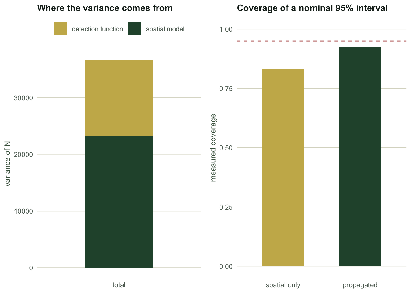
The detection function contributes `r sprintf("%.0f%%", 100 * p313_share)` of the total variance. That coefficient of variation on `p`, which looked negligible, is a *multiplier on every cell of the surface at once*. It does not average out across the region the way segment-level Poisson noise does, because it is the same error everywhere. Stage two's variance is a sum of many small independent errors; stage one's is one error applied to everything.
## Does it matter? Coverage says yes
Arguing about variance formulae is less useful than running the survey three hundred times and counting.
```{r mc}
one_dsm <- function(sv) {
  d <- sv$obs$dist
  f1 <- optim(log(0.1), function(ls) {
    s <- exp(ls); sum(d^2) / (2 * s^2) + length(d) * log(esw_of(s))
  }, method = "BFGS", hessian = TRUE)
  sg <- exp(f1$par); esw <- esw_of(sg); p <- esw / W
  se_sg <- sg * sqrt(1 / f1$hessian[1, 1])
  gr <- (esw_of(sg * 1.001) - esw_of(sg * 0.999)) / (0.002 * sg)
  se_p <- abs(gr) * se_sg / W
  sg2 <- expand.grid(line = lines_x, y0 = seq(0, 18, by = 2))
  sg2$ymid <- sg2$y0 + 1
  sg2$n <- mapply(function(lx, y0)
    sum(sv$obs$line == lx & sv$obs$y >= y0 & sv$obs$y < y0 + 2), sg2$line, sg2$y0)
  sg2$area <- 2 * esw * 2
  mm <- try(gam(n ~ s(line, ymid, k = 20), offset = log(area), family = poisson,
                data = sg2, method = "REML"), silent = TRUE)
  if (inherits(mm, "try-error")) return(NULL)
  gr2 <- expand.grid(line = seq(0.5, 29.5, 1), ymid = seq(0.5, 19.5, 1)); gr2$area <- 1
  l2 <- predict(mm, newdata = gr2, type = "link")
  Nh <- sum(exp(l2))
  Xm <- predict(mm, newdata = gr2, type = "lpmatrix")
  dN <- as.numeric(t(exp(l2)) %*% Xm)
  vsp <- as.numeric(t(dN) %*% vcov(mm) %*% dN)
  c(N = Nh, se_sp = sqrt(vsp), se_tot = sqrt(vsp + (Nh / p)^2 * se_p^2), Nt = sv$N_true)
}
M <- 300
res <- t(sapply(1:M, function(i) {
  r <- one_dsm(sim_survey(0.10, 5000 + i))
  if (is.null(r)) rep(NA_real_, 4) else r
}))
res <- res[complete.cases(res), ]
p313_M <- nrow(res)
p313_bias <- 100 * (mean(res[, "N"] / res[, "Nt"]) - 1)
p313_truecv <- sd(res[, "N"]) / mean(res[, "N"])
p313_mcv_sp <- mean(res[, "se_sp"] / res[, "N"])
p313_mcv_tot <- mean(res[, "se_tot"] / res[, "N"])
p313_cov_naive <- mean(abs(res[, "N"] - res[, "Nt"]) <= 1.96 * res[, "se_sp"])
p313_cov_prop <- mean(abs(res[, "N"] - res[, "Nt"]) <= 1.96 * res[, "se_tot"])
data.frame(replicates = p313_M,
           rel_bias_pct = p313_bias,
           cv_actual = p313_truecv,
           cv_spatial_only = p313_mcv_sp,
           cv_propagated = p313_mcv_tot,
           cover_spatial_only = p313_cov_naive,
           cover_propagated = p313_cov_prop)
```
The point estimate is fine: `r sprintf("%+.2f%%", p313_bias)` relative bias across `r p313_M` replicates. Nothing is wrong with the abundance number.
The intervals are another story. Across replicates the estimate actually varies with a coefficient of variation of `r sprintf("%.3f", p313_truecv)`. The spatial-only formula reports `r sprintf("%.3f", p313_mcv_sp)`, and a nominal 95% interval built on it covered the truth in `r sprintf("%.1f%%", 100 * p313_cov_naive)` of these replicates. Propagating the detection variance gets you to `r sprintf("%.3f", p313_mcv_tot)` and `r sprintf("%.1f%%", 100 * p313_cov_prop)`.
```{r fig-coverage}
#| echo: false
#| fig-cap: "Left: the two variance components. Right: measured coverage of nominal 95% intervals across 300 simulated surveys, with and without the detection term."
#| fig-alt: "Two panels. Left panel: one stacked bar showing the spatial variance component as the larger share and the detection component as roughly a third of the total. Right panel: two bars for measured coverage, the spatial-only bar reaching about 0.83 and the propagated bar reaching about 0.92, with a dashed line at the nominal 0.95."
vc <- data.frame(part = c("spatial model", "detection function"),
v = c(p313_vsp, p313_vdet))
vc$part <- factor(vc$part, levels = c("detection function", "spatial model"))
pA <- ggplot(vc, aes(x = "total", y = v, fill = part)) +
geom_col(width = 0.5) +
scale_fill_manual(values = c("spatial model" = "#275139",
"detection function" = "#c9b458")) +
labs(title = "Where the variance comes from", x = NULL, y = "variance of N") +
theme_te() + theme(legend.position = "top", legend.title = element_blank(),
panel.grid.major.y = element_line(colour = "#dad9ca", linewidth = 0.3))
cv <- data.frame(what = c("spatial only", "propagated"),
cover = c(p313_cov_naive, p313_cov_prop))
cv$what <- factor(cv$what, levels = c("spatial only", "propagated"))
pB <- ggplot(cv, aes(what, cover, fill = what)) +
geom_col(width = 0.55) +
geom_hline(yintercept = 0.95, linetype = "dashed", colour = "#b5534e", linewidth = 0.5) +
scale_fill_manual(values = c("spatial only" = "#c9b458", "propagated" = "#275139"),
guide = "none") +
scale_y_continuous(limits = c(0, 1)) +
labs(title = "Coverage of a nominal 95% interval", x = NULL, y = "measured coverage") +
theme_te() + theme(panel.grid.major.y = element_line(colour = "#dad9ca", linewidth = 0.3))
grid::grid.newpage()
grid::pushViewport(grid::viewport(layout = grid::grid.layout(1, 2)))
print(pA, vp = grid::viewport(layout.pos.row = 1, layout.pos.col = 1))
print(pB, vp = grid::viewport(layout.pos.row = 1, layout.pos.col = 2))
```
A survey you would report as plus or minus `r sprintf("%.0f", 100 * p313_mcv_sp)` per cent is really plus or minus roughly `r sprintf("%.0f", 100 * p313_mcv_tot)` to `r sprintf("%.0f", 100 * p313_truecv)` (the propagated figure and the spread across replicates, itself a Monte Carlo estimate). That is the difference between a population that has declined and one that has not.
## How close the propagated interval comes to 95%
Look again: `r sprintf("%.1f%%", 100 * p313_cov_prop)`, not 95. The propagation fixed most of the measured gap, and with `r p313_M` replicates the rest may be simulation noise: the Monte Carlo standard error of a coverage near this value is about `r sprintf("%.1f", 100 * sqrt(p313_cov_prop * (1 - p313_cov_prop) / p313_M))` percentage points.
Two things are still left out of the propagated interval, though neither is measured here. First, the GAM's covariance matrix is conditional on the smoothing parameter, which was itself estimated; the extra uncertainty from choosing how wiggly the surface is does not appear in `vcov(m)`. This is a known property of the Bayesian covariance matrix and it always points the same way, towards intervals that are too narrow.
Second, the target is moving. The true abundance in each replicate is a draw from a point process, not a constant, so an interval for the expected abundance is not automatically an interval for the realised one. Which of the two you want is a question about the survey, and the answer changes the arithmetic.
Neither of these is a reason to skip the propagation, and going from `r sprintf("%.0f%%", 100 * p313_cov_naive)` to `r sprintf("%.0f%%", 100 * p313_cov_prop)` may be all of the repair this simulation needs. Each is a reason not to describe the propagated interval as exact.
## What the model does not know
The surface between the lines is interpolation. Look at the figure again: the model saw ten vertical strips and painted the whole region. Nothing in the fit, the deviance explained, or the confidence band distinguishes a real gap between lines from a smoothing artefact, and the coverage above is measured on a surface that is genuinely smooth. On a patchy one it would be worse, and the model would not say so.
The other silence is more specific to distance sampling. Everything here assumes detection on the line is certain and that animals do not move in response to the observer. Break either and the whole surface scales by the wrong constant, quietly and everywhere. Those assumptions belong to stage one, and they are [tested where they live](../checking-a-distance-sampling-model/).
## Where to go next
If detection varies with something you measured, that belongs in stage one, not stage two: see [covariates in the detection function](../covariates-in-the-detection-function/). If you would rather fit both stages in one likelihood and let the uncertainty propagate itself, that is [hierarchical distance sampling](../hierarchical-distance-sampling/), which trades the flexible spatial smooth for a coherent variance. The choice between them is genuinely open. What is not open is reporting a DSM interval from the GAM alone.
## References
Hedley & Buckland 2004 Journal of Agricultural, Biological, and Environmental Statistics 9(2):181-199 (10.1198/1085711043578)
Miller, Burt, Rexstad & Thomas 2013 Methods in Ecology and Evolution 4(11):1001-1010 (10.1111/2041-210X.12105)
Johnson, Laake & Ver Hoef 2010 Biometrics 66(1):310-318 (10.1111/j.1541-0420.2009.01265.x)
Wood 2011 Journal of the Royal Statistical Society Series B 73(1):3-36 (10.1111/j.1467-9868.2010.00749.x)
Wood 2017 Generalized Additive Models: An Introduction with R, 2nd edition, ISBN 978-1-4987-2833-1
## Related tutorials
- [Line transect distance sampling in R](../distance-sampling-line-transect/)
- [Hierarchical distance sampling in R](../hierarchical-distance-sampling/)
- [Covariates in the detection function](../covariates-in-the-detection-function/)
- [Checking a distance sampling model](../checking-a-distance-sampling-model/)