---
title: "Correlated random walks and net displacement"
description: "Simulate correlated, bounded and directed random walks in R, and use net squared displacement to tell ranging apart from a bounded home range or a migration."
date: "2026-07-09 12:00"
categories: [R, movement ecology, random walk, simulation, ecology tutorial]
image: thumbnail.png
image-alt: "Three simulated movement paths from a common origin: a compact bounded path, a wandering correlated path, and a directed path heading off to one side."
---
The correlated random walk (CRW) is the default null model for animal movement: steps of random length with turning angles that favour keeping the current heading, so the path has directional persistence but no overall goal. The question that makes it useful is what a real track does relative to this baseline. Net squared displacement (NSD), the squared straight-line distance from the start, is the diagnostic. A freely ranging animal diffuses and its NSD grows about linearly; an animal confined to a home range has an NSD that plateaus; a migrating animal has an NSD that climbs faster than linear. This post simulates all three in base R and reads them off the NSD curve.
## Three regimes from one walk generator
We build one function that lays down a walk with gamma-distributed steps and persistent turning, and optionally adds a pull toward the origin (a home range) or a constant directional bias (a migration). Everything else is held equal, so only the bias distinguishes the regimes. The data are illustrative.
```{r}
#| label: setup
#| include: false
te_ink <- "#16241d"; te_body <- "#2c3a31"; te_forest <- "#275139"
te_label <- "#46604a"; te_sage <- "#93a87f"; te_paper <- "#f5f4ee"
te_line <- "#dad9ca"; te_faint <- "#5d6b61"; te_gold <- "#cda23f"; te_red <- "#b5534e"
theme_te <- function(base_size = 12) {
ggplot2::theme_minimal(base_size = base_size) +
ggplot2::theme(
text = ggplot2::element_text(colour = te_body),
plot.title = ggplot2::element_text(colour = te_ink, face = "bold"),
plot.subtitle = ggplot2::element_text(colour = te_faint),
axis.title = ggplot2::element_text(colour = te_label),
axis.text = ggplot2::element_text(colour = te_faint),
panel.grid.major = ggplot2::element_line(colour = te_line, linewidth = 0.3),
panel.grid.minor = ggplot2::element_blank(),
plot.background = ggplot2::element_rect(fill = te_paper, colour = NA),
panel.background = ggplot2::element_rect(fill = te_paper, colour = NA),
legend.key = ggplot2::element_blank(),
legend.title = ggplot2::element_text(colour = te_label),
strip.text = ggplot2::element_text(colour = te_ink, face = "bold"))
}
```
```{r}
#| label: sim
#| message: false
library(ggplot2); library(dplyr); library(tidyr)

sim_walk <- function(n, seed, mode = c("crw", "bounded", "directed"),
                     sigma_turn = 0.6, D = 12, wdir = 0.12) {
  mode <- match.arg(mode)
  set.seed(seed)
  sl <- rgamma(n, shape = 2, scale = 1)
  x <- y <- numeric(n + 1)
  heading <- runif(1, 0, 2 * pi)
  for (t in 1:n) {
    heading <- heading + rnorm(1, 0, sigma_turn)          # persistence
    if (mode == "bounded") {                              # pull home grows with distance
      d <- sqrt(x[t]^2 + y[t]^2); w <- min(1, d / D)
      b <- atan2(-y[t], -x[t])
      heading <- atan2((1 - w) * sin(heading) + w * sin(b),
                       (1 - w) * cos(heading) + w * cos(b))
    } else if (mode == "directed") {                      # constant bias toward +x
      heading <- atan2((1 - wdir) * sin(heading) + wdir * sin(0),
                       (1 - wdir) * cos(heading) + wdir * cos(0))
    }
    x[t + 1] <- x[t] + sl[t] * cos(heading)
    y[t + 1] <- y[t] + sl[t] * sin(heading)
  }
  data.frame(step = 0:n, x = x, y = y)
}

n <- 300
ex_crw <- sim_walk(n, 21, "crw")
ex_bnd <- sim_walk(n, 21, "bounded")
ex_dir <- sim_walk(n, 21, "directed")
round(c(crw = sqrt(tail(ex_crw$x, 1)^2 + tail(ex_crw$y, 1)^2),
        bounded = sqrt(tail(ex_bnd$x, 1)^2 + tail(ex_bnd$y, 1)^2),
        directed = sqrt(tail(ex_dir$x, 1)^2 + tail(ex_dir$y, 1)^2)), 1)
```
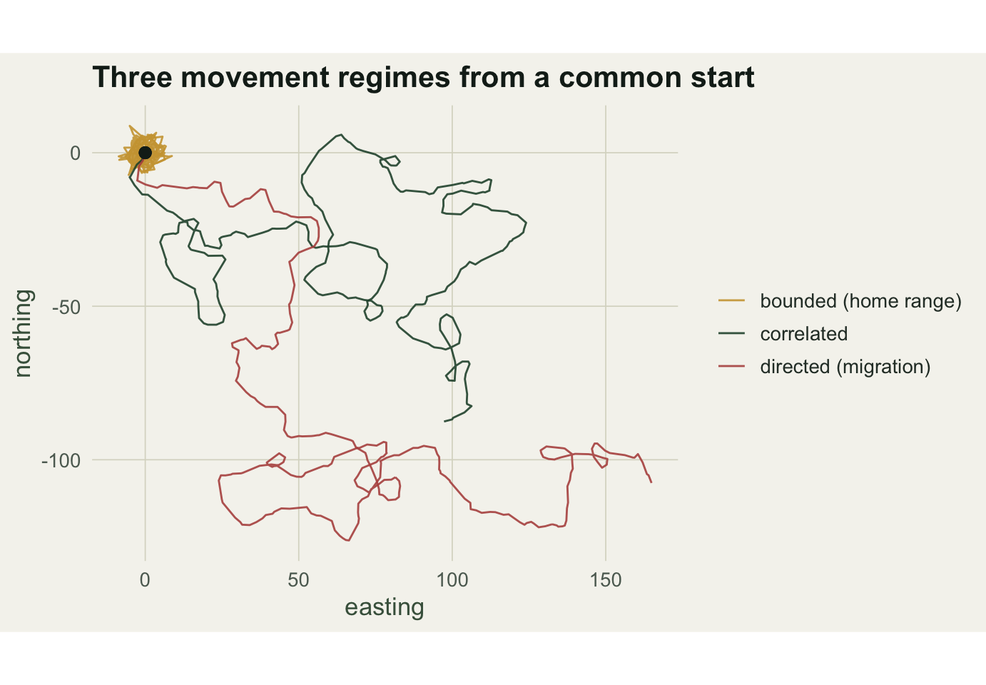
After 300 steps the correlated walk sits 131 units from the start and the directed walk 197, while the bounded walk has returned to within 4 units: the pull home keeps cancelling the wandering. Same steps, same turning, very different endpoints.
```{r}
#| label: fig-trajectories
#| fig-cap: "One walk of each regime from a common origin (black point). The bounded walk stays local, the correlated walk wanders, the directed walk leaves."
#| fig-alt: "Three paths from a shared start: a compact gold path near the origin, a green path wandering to one region, and a red path travelling steadily to the right."
#| fig-width: 7.2
#| fig-height: 5
traj <- rbind(cbind(ex_crw, regime = "correlated"),
              cbind(ex_bnd, regime = "bounded (home range)"),
              cbind(ex_dir, regime = "directed (migration)"))
traj$regime <- factor(traj$regime,
  levels = c("bounded (home range)", "correlated", "directed (migration)"))
ggplot(traj, aes(x, y, colour = regime)) +
  geom_path(linewidth = 0.5, alpha = 0.9) +
  geom_point(data = subset(traj, step == 0), size = 2.4, colour = te_ink) +
  scale_colour_manual(values = c("bounded (home range)" = te_gold,
                                 "correlated" = te_forest,
                                 "directed (migration)" = te_red), name = NULL) +
  coord_equal() +
  labs(title = "Three movement regimes from a common start", x = "easting", y = "northing") +
  theme_te(13)
```
## Net squared displacement and the diffusion null
NSD at step t is the squared distance from the origin. For a single walk it is noisy, so we average it over many replicate walks of each regime. For the correlated walk there is also an analytic expectation, derived by Kareiva and Shigesada (1983), that depends only on the mean and mean square of the step length and the mean cosine of the turning angle.
```{r}
#| label: nsd
mean_nsd <- function(mode, reps = 1000) {
  M <- matrix(0, reps, n + 1)
  for (r in 1:reps) {
    w <- sim_walk(n, 5000 + r, mode)
    M[r, ] <- w$x^2 + w$y^2
  }
  colMeans(M)
}
nsd_crw <- mean_nsd("crw"); nsd_bnd <- mean_nsd("bounded"); nsd_dir <- mean_nsd("directed")

s1 <- 2; s2 <- 2 * 1 + (2 * 1)^2           # E[l] = 2, E[l^2] = var + mean^2 = 6
cc <- exp(-0.6^2 / 2)                       # mean cosine of the turning angle
ks <- function(k) k * s2 + 2 * s1^2 * (cc / (1 - cc)) * (k - (1 - cc^k) / (1 - cc))
ks_vals <- sapply(0:n, ks)

round(c(mean_cosine = cc, nsd_crw = nsd_crw[n + 1], ks = ks_vals[n + 1],
        crw_ks_ratio = nsd_crw[n + 1] / ks_vals[n + 1],
        nsd_bounded = nsd_bnd[n + 1], nsd_directed = nsd_dir[n + 1]), 3)
```
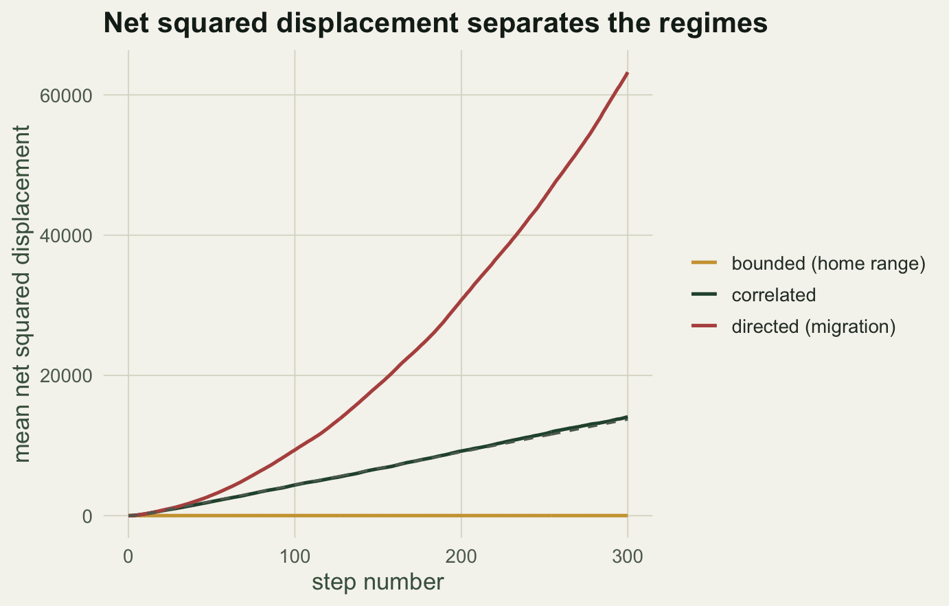
The mean cosine of the turning angle is 0.835, which sets the persistence. At step 300 the correlated walk reaches a mean NSD of about 14090, within 3% of the Kareiva-Shigesada value of 13720: the correlated walk is doing exactly what the diffusion null predicts. The bounded walk sits at 19, having stopped spreading, and the directed walk is at 63240, more than four times the correlated one.
```{r}
#| label: fig-nsd
#| fig-cap: "Mean net squared displacement by regime, with the Kareiva-Shigesada expectation for the correlated walk (dashed). Bounded plateaus, correlated grows linearly on the null, directed climbs faster."
#| fig-alt: "Net squared displacement against step: a flat gold curve near zero, a green curve rising linearly with a dashed line lying on top of it, and a red curve rising faster and curving upward."
#| fig-width: 7.2
#| fig-height: 4.6
steps <- 0:n
nd <- rbind(
  data.frame(step = steps, nsd = nsd_bnd, regime = "bounded (home range)"),
  data.frame(step = steps, nsd = nsd_crw, regime = "correlated"),
  data.frame(step = steps, nsd = nsd_dir, regime = "directed (migration)"))
nd$regime <- factor(nd$regime,
  levels = c("bounded (home range)", "correlated", "directed (migration)"))
ggplot(nd, aes(step, nsd, colour = regime)) +
  geom_line(linewidth = 0.9) +
  geom_line(data = data.frame(step = steps, nsd = ks_vals), aes(step, nsd),
            colour = te_faint, linetype = "dashed", linewidth = 0.6, inherit.aes = FALSE) +
  scale_colour_manual(values = c("bounded (home range)" = te_gold,
                                 "correlated" = te_forest,
                                 "directed (migration)" = te_red), name = NULL) +
  labs(title = "Net squared displacement separates the regimes", x = "step number",
       y = "mean net squared displacement") +
  theme_te(13)
```
## Reading the growth rate
The clearest summary is the diffusion exponent: the slope of NSD against step on log-log axes. A plateau gives a slope near zero, ordinary diffusion gives one, and straight-line travel gives two.
```{r}
#| label: exponent
half <- (n / 2):n
slope <- function(v) coef(lm(log(v[half + 1]) ~ log(half)))[2]
round(c(bounded = slope(nsd_bnd), correlated = slope(nsd_crw), directed = slope(nsd_dir)), 2)
```
The exponents come out near zero for the bounded walk, close to one for the correlated walk, and near two for the directed walk. That single number is what NSD-based methods use to classify tracks into resident, ranging, or migratory movement (Bunnefeld 2011). It also connects the earlier posts: a plateauing NSD is the signature of the bounded use that a home-range estimator summarises, and a straight-line NSD is the freely diffusing case where a kernel range keeps growing with tracking effort.
## What to take away
The correlated random walk is the reference against which movement is read, and its expected displacement has a closed form (Kareiva 1983; Bovet 1988). Net squared displacement turns that reference into a diagnostic: near-zero growth means a bounded home range, linear growth means diffusive ranging on the null, and faster-than-linear growth means directed movement. Two cautions carry over from the rest of this series. Telling a bounded walk from a slowly diffusing one needs a long enough track, because early on a plateau and slow growth look alike, so a short series is not enough to rule out ranging. And the persistence that drives the whole picture depends on the fix interval, so the same animal sampled at a coarser rate will look less correlated and more diffusive. Movement summaries are only interpretable with the sampling design stated alongside them.
## References
Kareiva & Shigesada 1983 Oecologia 56(2-3):234-238 (10.1007/BF00379695)
Bovet & Benhamou 1988 Journal of Theoretical Biology 131(4):419-433 (10.1016/S0022-5193(88)80038-9)
Turchin 1998 Quantitative Analysis of Movement, Sinauer Associates, ISBN 978-0-87893-847-8
Bunnefeld, Borger, van Moorter, Rolandsen, Dettki, Solberg & Ericsson 2011 Journal of Animal Ecology 80(2):466-476 (10.1111/j.1365-2656.2010.01776.x)
Codling, Plank & Benhamou 2008 Journal of the Royal Society Interface 5(25):813-834 (10.1098/rsif.2008.0014)
## Related tutorials
- [Step lengths and turning angles](../step-lengths-turning-angles/)
- [Home ranges: MCP versus kernel density](../home-range-mcp-kde/)
- [Resource selection functions](../resource-selection-functions/)
- [Complete spatial randomness and quadrat tests](../complete-spatial-randomness-quadrat/)