library(ggplot2)
library(dplyr)
library(tidyr)

ink <- "#16241d"; body <- "#2c3a31"; forest <- "#275139"; gold <- "#c9b458"
paper <- "#f5f4ee"; line_c <- "#dad9ca"; faint <- "#5d6b61"; sage <- "#93a87f"; red <- "#b5534e"

theme_te <- function(base = 12) {
  theme_minimal(base_size = base) +
    theme(panel.grid.minor = element_blank(),
          panel.grid.major = element_line(colour = line_c, linewidth = 0.3),
          plot.background = element_rect(fill = paper, colour = NA),
          panel.background = element_rect(fill = paper, colour = NA),
          axis.title = element_text(colour = body), axis.text = element_text(colour = faint),
          plot.title = element_text(colour = ink, face = "bold"),
          plot.subtitle = element_text(colour = faint),
          legend.title = element_text(colour = body), legend.text = element_text(colour = faint))
}Closed-population capture-recapture in R
R
abundance
detection
ecology tutorial
Estimate the size of a closed population from repeated capture occasions. Fit Lincoln-Petersen, Schnabel and the model M0 likelihood from scratch in R.
Mark the animals you catch, release them, and catch again. The fraction of your later catch that is already marked tells you how large the population is: if most captures are recaptures, you have already found most of the animals, and if few are, many remain unseen. Counting only the distinct individuals you handled gives a firm lower bound, never the total, because some animals are never caught at all.
Capture-recapture turns the recapture rate into an estimate of that unseen fraction. This post starts with the two-sample Lincoln-Petersen estimator and its bias correction, moves to the Schnabel estimator for many occasions, and then fits the full model M0 likelihood by hand with optim. The theme running through all three is the same one behind the occupancy and N-mixture posts: the count you see is not the population, and the structure of repeated sampling lets you recover what you missed.
Two samples: Lincoln-Petersen and Chapman
The oldest idea, from Petersen (1896) and Lincoln (1930), uses two occasions. Mark n1 animals on the first, then on the second catch n2 animals of which m2 are already marked. If marks mix evenly through the population, the marked fraction of the second sample should match the marked fraction of the whole, giving
\[\hat{N} = \frac{n_1 n_2}{m_2}.\]
This ratio is biased upward, badly so when m2 is small, because a small denominator swings the estimate. Chapman (1951) gives an almost unbiased version by adding one to each count,
\[\hat{N}_{C} = \frac{(n_1 + 1)(n_2 + 1)}{m_2 + 1} - 1,\]
which is the form to use in practice.
The model M0
With more than two occasions we can do better. Model M0 assumes every animal is caught on every occasion with the same probability p, independently. Over k occasions an animal is never caught with probability (1 - p)^k, so if M distinct animals are seen and n captures are made in total, the likelihood in N and p is
\[L(N, p) \propto \frac{N!}{(N - M)!}\; p^{n} (1 - p)^{kN - n}.\]
The number of distinct animals seen and the total number of captures are all the model needs. We fit it by profiling: fix a candidate N, take the best p for it, and keep the N that maximises the likelihood.
Simulating a study
We mark a closed population of 300 animals over five occasions with a per-occasion catch probability of 0.25. Each animal’s capture history is a row of Bernoulli draws.
set.seed(18)
Ntrue <- 300; p_true <- 0.25; k <- 5

H <- matrix(rbinom(Ntrue * k, 1, p_true), Ntrue, k)  # capture histories, one row per animal
seen <- rowSums(H) > 0
Mt1 <- sum(seen)     # distinct animals ever caught
n <- sum(H)          # total number of captures
c(distinct_seen = Mt1, total_captures = n, never_seen = Ntrue - Mt1)
distinct_seen total_captures never_seen
229 371 71 Across five occasions we handle 229 distinct animals and make 371 captures. Those 229 are a lower bound on the population: 71 animals were never caught even once, and no amount of counting the marked ones would reveal them. Everything below is about estimating those 71.
The accumulation of distinct individuals
Track how many animals are seen for the first time on each occasion. The count of new animals falls as the marked pool grows, and the running total of distinct individuals climbs toward, but never reaches, the true population.
newly <- integer(k); cumd <- integer(k); everseen <- logical(Ntrue)
for (t in 1:k) {
  newthis <- H[, t] == 1 & !everseen
  newly[t] <- sum(newthis)
  everseen <- everseen | H[, t] == 1
  cumd[t] <- sum(everseen)
}
rbind(newly = newly, cumulative = cumd)
[,1] [,2] [,3] [,4] [,5]
newly 67 56 44 35 27
cumulative 67 123 167 202 229d1 <- data.frame(occ = 1:k, newly = newly, cum = cumd)
ggplot(d1, aes(occ)) +
geom_col(aes(y = newly), width = 0.55, fill = sage) +
geom_line(aes(y = cum), colour = forest, linewidth = 0.9) +
geom_point(aes(y = cum), colour = forest, size = 2.4) +
geom_hline(yintercept = Ntrue, linetype = "dashed", colour = red, linewidth = 0.5) +
annotate("text", x = 1.1, y = Ntrue + 9, label = "true N = 300", colour = red, hjust = 0, size = 3.4) +
labs(title = "New captures fall but never reach the true total",
subtitle = "Newly marked animals per occasion (bars) and cumulative distinct caught (line)",
x = "Capture occasion", y = "Individuals") +
theme_te()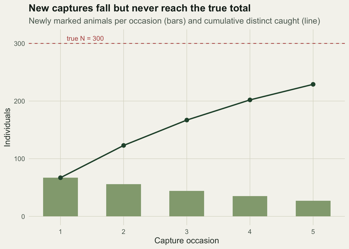
The number of new animals drops from 67 on the first occasion to 27 on the fifth. The gap between the flattening curve and the dashed line at 300 is exactly what the estimators have to fill in.
The three estimators
First the two-sample estimators, using only occasions one and two.
n1 <- sum(H[, 1]); n2 <- sum(H[, 2]); m2 <- sum(H[, 1] == 1 & H[, 2] == 1)
Nlp <- n1 * n2 / m2
Nch <- (n1 + 1) * (n2 + 1) / (m2 + 1) - 1
var_ch <- (n1 + 1) * (n2 + 1) * (n1 - m2) * (n2 - m2) / ((m2 + 1)^2 * (m2 + 2))
se_ch <- sqrt(var_ch)
c(n1 = n1, n2 = n2, m2 = m2, Lincoln_Petersen = Nlp, Chapman = Nch,
  lo = Nch - 1.96 * se_ch, hi = Nch + 1.96 * se_ch)
n1 n2 m2 Lincoln_Petersen
67.0000 71.0000 15.0000 317.1333
Chapman lo hi
305.0000 192.8167 417.1833 With only 15 animals recaptured between the two occasions, Lincoln-Petersen returns 317 and the Chapman correction pulls it to 305, but the interval is enormous, roughly 193 to 417. Two occasions simply do not carry much information. The Schnabel estimator uses all five, accumulating the marked pool as it goes.
caught_before <- 0; num <- 0; den <- 0
for (t in 1:k) {
  Ct <- sum(H[, t])                  # caught on occasion t
  Mt <- caught_before                # marked animals already in the population
  Rt <- if (t == 1) 0 else sum(H[, t] == 1 & rowSums(H[, 1:(t-1), drop = FALSE]) > 0)
  num <- num + Ct * Mt
  den <- den + Rt
  caught_before <- sum(rowSums(H[, 1:t, drop = FALSE]) > 0)
}
Nsch <- num / den
se_inv <- sqrt(den) / num; inv <- den / num     # interval on 1/N, then inverted
sch_ci <- 1 / (inv + c(1.96, -1.96) * se_inv)
c(N_schnabel = Nsch, lo = sch_ci[1], hi = sch_ci[2])
N_schnabel lo hi
301.0986 258.5692 360.3725 Schnabel gives 301 with an interval of about 259 to 360, far tighter than the two-sample result because every occasion adds recaptures. Finally the model M0 likelihood, fitted by profiling over integer N.
Ngrid <- Mt1:(Mt1 + 600)
ll <- sapply(Ngrid, function(N) {
  p <- n / (k * N)                    # closed-form best p for this N
  if (p <= 0 || p >= 1) return(-Inf)
  lgamma(N + 1) - lgamma(N - Mt1 + 1) + n * log(p) + (k * N - n) * log(1 - p)
})
NhatM0 <- Ngrid[which.max(ll)]
cut <- max(ll) - qchisq(0.95, 1) / 2
ciM0 <- range(Ngrid[ll >= cut])
c(N_M0 = NhatM0, lo = ciM0[1], hi = ciM0[2], p = n / (k * NhatM0))
N_M0 lo hi p
303.0000000 278.0000000 335.0000000 0.2448845 Model M0 estimates 303 individuals with an interval of 278 to 335 and a catch probability of 0.25, matching the truth. It is the most precise of the three because it uses the full pattern of capture histories rather than summary counts.
d2 <- data.frame(
  method = factor(c("Distinct seen\n(lower bound)", "Lincoln-Petersen\n(Chapman)", "Schnabel", "Model M0"),
                  levels = c("Distinct seen\n(lower bound)", "Lincoln-Petersen\n(Chapman)", "Schnabel", "Model M0")),
  est = c(Mt1, Nch, Nsch, NhatM0),
  lo = c(NA, Nch - 1.96 * se_ch, sch_ci[1], ciM0[1]),
  hi = c(NA, Nch + 1.96 * se_ch, sch_ci[2], ciM0[2]),
  grp = c("seen", "est", "est", "est"))

ggplot(d2, aes(method, est, colour = grp)) +
  geom_hline(yintercept = Ntrue, linetype = "dashed", colour = faint) +
  geom_errorbar(aes(ymin = lo, ymax = hi), width = 0.14, linewidth = 0.7, na.rm = TRUE) +
  geom_point(size = 3.2) +
  scale_colour_manual(values = c(seen = gold, est = forest), guide = "none") +
  annotate("text", x = 0.7, y = Ntrue + 7, label = "truth", colour = faint, hjust = 0, size = 3.3) +
  labs(title = "Capture-recapture recovers the animals never seen",
       subtitle = "Population estimates with 95% intervals against the simulation truth",
       x = NULL, y = "Estimated population size") +
  theme_te()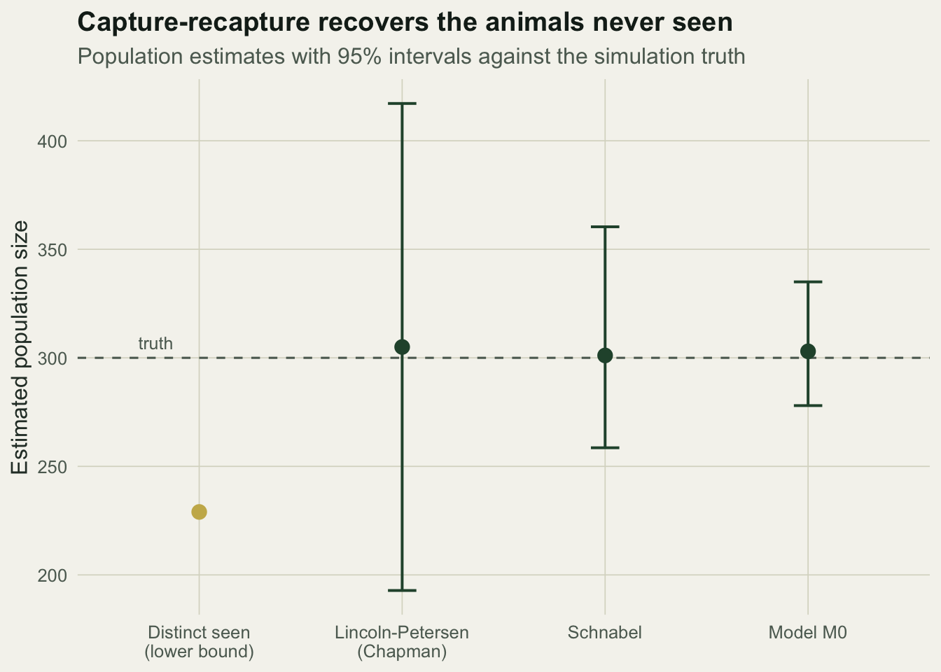
An interval for the population
As with removal sampling, the interval for a population size is asymmetric: the data rule out small populations more firmly than large ones. The profile likelihood for model M0 shows this shape directly.
d3 <- data.frame(N = Ngrid, rll = ll - max(ll))
d3 <- d3[d3$rll > -6, ]
ggplot(d3, aes(N, rll)) +
  annotate("rect", xmin = ciM0[1], xmax = ciM0[2], ymin = -Inf, ymax = Inf, alpha = 0.08, fill = gold) +
  geom_line(colour = forest, linewidth = 0.7) +
  geom_hline(yintercept = -qchisq(0.95, 1) / 2, linetype = "dashed", colour = faint) +
  geom_vline(xintercept = NhatM0, colour = red, linewidth = 0.5) +
  labs(title = "Profile likelihood for population size under model M0",
       subtitle = "Relative log-likelihood; dashed line is the 95% cut, shaded band the interval",
       x = "Population size N", y = "Relative log-likelihood") +
  theme_te()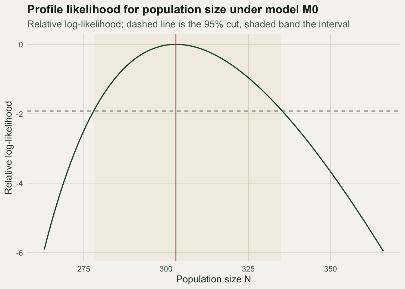
Assumptions and when it fails
All three estimators assume the population is closed, that marks are neither lost nor missed, and that every animal has the same catch probability. That last assumption is the fragile one. Otis and colleagues (1978) set out a family of models for the ways it breaks: real animals often differ in catchability, so trap-happy or trap-shy individuals distort the recapture rate, and capture on one occasion can change the probability of capture on the next. When catchability varies among individuals, the easy animals are caught repeatedly and the hard ones stay unseen, so M0 underestimates the population; their model Mh addresses this, Mt allows the probability to differ by occasion, and Mb allows a behavioural response to first capture. Fitting the wrong model gives a confident wrong answer, so choosing among them, rather than defaulting to M0, is the substance of a real analysis.
References
Chapman 1951 University of California Publications in Statistics 1(7):131-160 (pre-DOI monograph, University of California Press)
Schnabel 1938 American Mathematical Monthly 45(6):348-352 (10.1080/00029890.1938.11990818)
Otis, Burnham, White and Anderson 1978 Wildlife Monographs 62:3-135 (10.2307/3830650)